Numerical simulation of Oldroyd-B fluid with application to hemodynamics

Abstract

Oldroyd-B viscoelastic fluid is numerically simulated using the stabilized Galerkin least squares finite element method. The instabilities due to the connective nature of the Oldroyd-B model is treated using the discrete viscous elastic split stress method. The model is used to study the behavior of the flow of blood through an abdominal aortic segment. The results show that the viscoelastic nature of the blood should be considered specially at low shear rates.

Introduction

One of the most common problems which occur in the abdominal aortic artery is the abdominal aortic aneurysms (AAAs) where the artery has a balloon-shaped expansion, and hence, the increase in the lumen diameter reach to 50% of its normal diameter. ¹ One of the causes of the AAAs is the loss of arterial wall integrity. ² In men, it is found that AAA happens commonly in those above the fifth decade. ³

In this work, the geometry is considered as a two-dimensional (2D) planar channel with non-deformable walls. Although this assumption is less realistic than other assumptions such as axisymmetric or three-dimensional, this assumption is acceptable for geometries with spatial symmetry. There are many works for blood flow simulations that consider the assumption of planar channel for arteries.^4–7 Many studies^8–14 related to AAAs considered the blood as a purely viscous fluid with constant viscosity, that is, Newtonian fluid. In this work, the blood is modeled as a viscoelastic fluid where the Oldroyd-B constitutive model is used to represent the viscoelastic property of the blood.

The stabilized Galerkin least squares (GLS) method is used ¹⁵ since high Reynolds numbers are expected in blood flows. Due to lack of enough diffusion in the Oldroyd model, the discrete viscous elastic split stress (DEVSS) method ¹⁶ is used to suppress the associated instabilities. An in-house built FORTRAN code is built to solve the governing equations, and the results are visualized using the Techplot software. This article is organized as follows: the problem’s geometry is described in “Problem geometry” section while the governing equations and stabilization techniques are described in “Mathematical modeling,”“The incompressiblity constraint,” and “The DEVSS method” sections. Numerical parameters of the problem are stated in “Numerical simulation” section. Finally, results are presented and discussed in “Results and discussion” section.

Problem geometry

Figure 1 describes the upper half of geometry used in the current work in which a 2D channel with single aneurysm is considered. Equation (1) is the mathematical description of the upper wall geometry ¹³

$$y=\{\begin{array}{cc}\frac{D}{2}\hfill & 0\le x\le L_1\hfill \\ \multicolumn{1}{c}{\left(\frac{D_1-D}{4}\right)[1+\sin (\frac{2\pi (x-L_1)}{L_2}-\frac{\pi }{2})]+\frac{D}{2}}& L_1\le x\le L_2\hfill \\ \multicolumn{1}{c}{\frac{D}{2}}& L_2\le x\le L_T\hfill \end{array}$$

(1)

in which $D$ is the artery diameter at the inlet section and $L_T$ is the artery length with $L_1=2.5D$ , $L_2=5D$ , $L_{\mathrm{T}}=7.5D$ , and $D_1=2D$ . In this study, the diameter of the artery is taken to be 8 mm. ¹³

Figure 1.

Geometry of the artery.

Mathematical modeling

Balance laws

Considering non-polar incompressible, viscous fluids, the balance of linear momentum is

$$\rho (\frac{\partial \mathbf{V}}{\partial t}+\nabla ·(\mathbf{V}\otimes \mathbf{V}))=-\nabla p+{\mu }_s\mathrm{\Delta }\mathbf{V}+\nabla ·{\mathbf{\tau }}_p$$

(2)

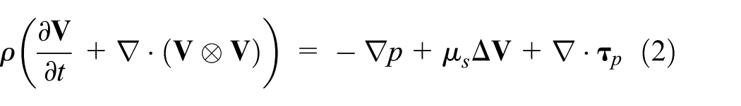
and the continuity equation reads

$$\nabla ·\mathbf{V}=0$$

(3)

where $\rho$ is the fluid density, $\mathbf{V}$ is the velocity vector, $p$ is the pressure, ${\mu }_s$ is the solvent zero-shear-rate viscosity, and ${\mathbf{\tau }}_p$ is the polymeric contribution to the extra stress tensor. For Newtonian fluids, ${\mathbf{\tau }}_p$ vanishes.

Constitutive laws

For viscoelastic fluids, the extra stress tensor is related to the velocity gradient via a differential equation. In the Oldroyd-B model, polymeric contribution is

$$\begin{array}{c}\lambda (\frac{\partial {\mathbf{\tau }}_p}{\partial t}+(\mathbf{V}·\nabla ){\mathbf{\tau }}_p-(\nabla \mathbf{V}){\mathbf{\tau }}_p-{\mathbf{\tau }}_p{(\nabla \mathbf{V})}^{\mathrm{T}})\hfill \\ +{\mathbf{\tau }}_p={\mu }_p(\nabla \mathbf{V}+{(\nabla \mathbf{V})}^{\mathrm{T}})\hfill \end{array}$$

(4)

where ${\mu }_p$ is the polymer zero-shear-rate viscosity and $\lambda$ is the relaxation time. ¹⁷

Nondimensionalization scheme

The following nondimensionalization scheme is used

$$\begin{array}{c}{x}^{*}=\frac{x}{D},y^{*}=\frac{y}{D},{\mathbf{V}}^{*}=\frac{\mathbf{V}}{V_m},t^{*}=\frac{t{V}_m}{D},\hfill \\ p^{*}=\frac{p-p_{\mathrm{exit}}}{\rho {V_m}^2}\mathrm{and}{\mathbf{\tau }}^{*}=\frac{\mathbf{\tau }}{\rho {V_m}^2}\hfill \end{array}$$

in which $V_m$ is the inlet average velocity and $p_{\mathrm{exit}}$ is the exit pressure. The velocity vector is $\mathbf{V}=(u,v)$ and the polymeric stress tensor is

$${\mathbf{\tau }}_p=\left[\begin{array}{cc}S\hfill & Q\hfill \\ \multicolumn{1}{c}{Q}& T\hfill \end{array}\right]$$

(5)

in which $S,Q,\mathrm{and}T$ are the axial, shear, and normal stresses, respectively. The non-dimensional form of equations (2) and (4) are (the asterisk is dropped for clarity)

$$\frac{\partial \mathbf{V}}{\partial t}+\nabla ·(\mathbf{V}\otimes \mathbf{V})=-\nabla p+\frac{\beta }{\mathrm{Re}}\mathrm{\Delta }\mathbf{V}+\nabla ·{\mathbf{\tau }}_p$$

(6)

$$\begin{array}{c}\frac{\partial {\mathbf{\tau }}_p}{\partial t}+(\mathbf{V}·\nabla ){\mathbf{\tau }}_p-(\nabla \mathbf{V}){\mathbf{\tau }}_p-{\mathbf{\tau }}_p{(\nabla \mathbf{V})}^{\mathrm{T}}+\frac{{\mathbf{\tau }}_p}{\mathrm{We}}\hfill \\ =\frac{(1-\beta )}{\mathrm{We}\mathrm{Re}}(\nabla \mathbf{V}+{(\nabla \mathbf{V})}^{\mathrm{T}})\hfill \end{array}$$

(7)

where $\mathrm{Re}=(\rho V_{m}D)/(\rho V_{m}D)\mu \mu$ is the Reynolds number, $\mu ={\mu }_s+{\mu }_p$ is the total viscosity, $\mathrm{We}=\lambda \left(V_m/V_{m}DD\right)$ is the Weissenberg number, and $\beta ={\mu }_s/{\mu }_s\mu \mu$ is the viscosity ratio.

The incompressiblity constraint

To recover the link between the continuity and momentum equations, a modified form of the continuity equation is used using the pressure stabilized technique ¹⁸

$$\nabla ·\mathbf{V}=\epsilon {\nabla }^{2}p$$

(8)

in which, $\epsilon$ is a controlling parameter used to stabilize the pressure. In this study, the value of stabilization parameter is chosen to be 0.0001, where the time step values range from 0.0001 to 0.00005 according to the value of Reynolds number. The main advantage with this technique is that equal order basis functions could be used for all primitive variables. ¹⁹

The DEVSS method

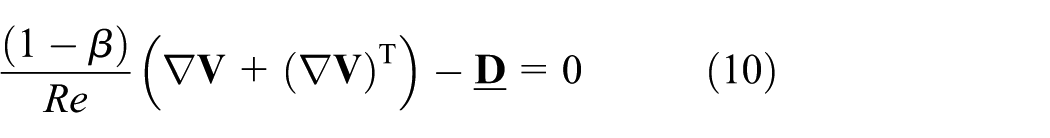
Since the additional polymeric stress induces numerical instabilities, ²⁰ the DEVSS method is used in which the discrete form of the momentum equation is modified by adding extra diffusion. Introduce the Newtonian-like stress tensor $\underset{¯}{\mathbf{D}}$ defined as $\underset{¯}{\mathbf{D}}={\mu }_p(\nabla \mathbf{V}+(\nabla \mathbf{V}{)}^{\mathrm{T}})$ to the momentum equation which leads to a symmetric influence matrix. The momentum equation, equation (2), is reformulated as follows

$$\begin{array}{c}\rho \frac{\partial \mathbf{V}}{\partial t}+\rho (\mathbf{V}·\nabla \mathbf{V})=-\nabla p+\nabla ·\hfill \\ ({\mu }_s(\nabla \mathbf{V}+{(\nabla \mathbf{V})}^{\mathrm{T}})+{\mathbf{\tau }}_p)+\nabla ·({\mu }_p(\nabla \mathbf{V}+{(\nabla \mathbf{V})}^{\mathrm{T}})-\underset{¯}{\mathbf{D}})\hfill \end{array}$$

(9)

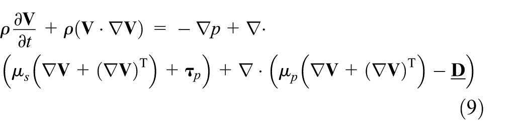
The extra variable $\underset{¯}{\mathbf{D}}$ can be calculated from the following non-dimensional equation

$$\frac{(1-\beta )}{\mathrm{Re}}(\nabla \mathbf{V}+{(\nabla \mathbf{V})}^{\mathrm{T}})-\underset{¯}{\mathbf{D}}=0$$

(10)

We can rewrite equation (9) in the non-dimensional form as follows

$$\begin{array}{c}\frac{\partial \mathbf{V}}{\partial t}+\nabla ·(\mathbf{V}\otimes \mathbf{V})=-\nabla p+\nabla ·\hfill \\ (\frac{\nabla \mathbf{V}+{(\nabla \mathbf{V})}^{\mathrm{T}}}{\mathrm{Re}}+{\mathbf{\tau }}_p-\underset{¯}{\mathbf{D}})\hfill \end{array}$$

(11)

This is the stabilized form of the balance of momentum equation.

Numerical simulation

The set of equations (7), (8), (10), and (11) are solved numerically using the finite elements method. The GLS technique is used in which the basis function is modified which leads to stable solutions. ¹⁰ The unsteady terms are discretized using the first-order explicit Euler scheme. The time step is chosen small enough to obtain accurate and stable solutions. Zero values for the flow variables are used as an initial guess.

Numerical parameters

The physiological condition^21–23 described in Table 1 is used in the current work.

Table 1.

Blood physiological conditions.

$\rho$	$1050\mathrm{kg}/{\mathrm{m}}^3$	${\mu }_{\mathrm{p}}$	$4\times {10}^{-4}\mathrm{Pa}\mathrm{s}$
${\mu }_{\mathbf{s}}$	$0.00319\mathrm{Pa}\mathrm{s}$	$\lambda$	$0.06\mathrm{s}$

Boundary conditions

The no-slip boundary condition is imposed over the walls. A fully developed flow is assumed at the artery inlet. At the artery exit, the normal component of the Cauchy stress tensor is set to zero, namely, the pressure, p, is set to zero as well as the normal stress T.

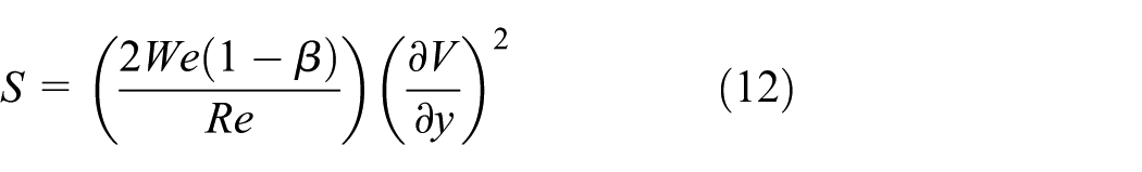
According to the theory of characteristics, two components of the stress have to be specified at the inlet. ¹⁷ Using the fully developed flow assumption at the inlet, the axial and shear stresses are^24,25

$$S=\left(\frac{2\mathrm{We}(1-\beta )}{\mathrm{Re}}\right){\left(\frac{\partial V}{\partial y}\right)}^2$$

(12)

$$Q=\left(\frac{(1-\beta )}{\mathrm{Re}}\right)\frac{\partial V}{\partial y}$$

(13)

Results and discussion

Results are obtained for both cases, namely, the Newtonian case $({\mathbf{\tau }}_p=0)$ and the viscoelastic case. In both cases, different values for the blood volumetric flow rate are considered as shown in Table 2. The corresponding Reynolds and Weissenberg numbers are described in Table 2 as well.

Table 2.

Blood volumetric flow rate and corresponding Reynolds and Weissenberg numbers.

Flow rate in cm3/s	$\mathrm{Re}$	$\mathrm{We}$
0.1	4.65	0.01492
0.5	23.27	0.0746
1	46.54	0.1492
2	93.09	0.2984
3	139.7	0.447

Grid-independent solution

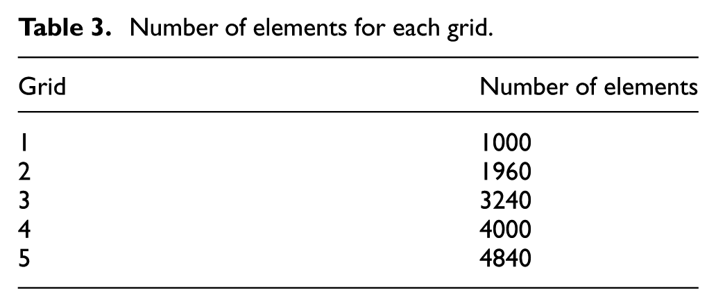
Different mesh sizes are used to reach the mesh-independent solution. The computational domain shown in Figure 2 is discretized using 4000 bilinear quadrilateral iso-parametric elements. Table 3 includes the number of elements for each grid. The wall shear stress (WSS) is calculated using all meshes for the volumetric flow rate Q = 3 cm³/s. Figure 3 shows that the last two solutions are very close to each other assuring that the finer the mesh, the better the solution.

Figure 2.

Computational domain.

Table 3.

Number of elements for each grid.

Grid	Number of elements
1	1000
2	1960
3	3240
4	4000
5	4840

Figure 3.

Grid-independent solution for WSS.

Viscoelastic flow patterns

Parametric study is performed to investigate the effect of the blood volumetric flow rate and, consequently, the Re and We on the velocity contours and the formulation of recirculation zones. In this study, the steady state solutions are considered. It is found that the time required for obtaining the steady solution is dependent on the Reynolds number. For example, the number of time steps for steady state for Q = 0.1 cm³/s is 10,000 and the time step in this case is 0.0001 while the number of time steps is 50,000 for Q = 1 cm³/s at the same time step. Figure 4 shows low Re flows in which there are no vortices as indicated in cases (a) and (b), and the main stream fills the aneurysm. The vortices begin to appear for higher Re, and it is noted that the vortex size increases with the increase of flow rate till it fills the entire aneurysm. The formulation of vortices proves to have a great effect on the integrity of the arterial wall. ²⁶

Figure 4.

Viscoelastic flow streamlines for different flow rates: (a) flow rate = 0.1 cm³/s, (b) flow rate = 0.5 cm³/s, (c) flow rate = 1 cm³/s, (d) flow rate = 2 cm³/s, and (e) flow rate = 3 cm³/s.

WSS distribution

The WSS, defined as the sum of the Newtonian contribution and the polymeric contribution, is one of the most important factors that affects the integrity of the arterial wall is the WSS. Boyd et al. ²⁶ found that the minimum values of the WSS have more substantial effect than large values. Figure 5 shows the spatial variation of the WSS for different flow rates. The minimum values for WSS occur in the region of the aneurysm due to the convective deceleration of the flow which results in small velocity gradients at the wall. ¹³ The WSS changes its sign from negative values within the aneurysm to positive sign at the distal end of the aneurysm at which it reaches its maximum values.

Figure 5.

Wall shear stress (WSS) distribution.

Wall pressure distribution

Another important factor in hemodynamics is the blood pressure distribution at the arterial wall shown in Figure 6 for different flow conditions. The pressure is decreasing downstream till it reaches the aneurysm region in which it starts to build up until it reaches it maximum, which is proportional to the flow rate; at the distal end, it starts to decrease again toward the artery exit.

Figure 6.

Wall pressure distribution.

Axial velocity

To have more insights into the blood flow through the abdominal aneurysms, it is convenient to calculate the axial velocity on a vertical line at the mid-section of the aneurysm for different flow rate conditions as shown in Figure 7.

Figure 7.

Axial velocity for different flow rates.

It is noted that the axial velocity increases with the increase of the Reynolds number due to the increase of the flow rate. The axial velocity takes negative values near the arterial wall, and these values appear clearly for high flow rates. This is due to the formation of the vortices which assert again that the aneurysm zone is a region which is worth to be studied.

Viscoelastic versus Newtonian flows

To show the importance of the inclusion of the viscoelasticity effects, the WSS is compared for both cases for different flow conditions. Figure 8 shows a difference of about 13% for the low flow rate case, while this difference reaches 40% in the distal end region of the aneurysm for higher flow rates as indicated in Figure 9.

Figure 8.

Comparison of the WSS for Q = 0.1 cm³/s.

Figure 9.

Comparison of the WSS for Q = 3 cm³/s.

This asserts that the effect of red blood cell in the blood flow simulation is important and should not be ignored, although there are many studies that treated the blood as a Newtonian fluid. This conclusion is consistent with Berger and Jou. ²⁷

Summary and conclusion

In this contribution, mathematical modeling and finite element analysis are presented for viscoelastic Oldroyd-B fluid. The model is used to simulate blood flow in a rigid artery. In order to simulate low shear rate conditions as well as high shear rates, different flow conditions are considered ranging from volumetric flowrate of 0.1–3 cm³/s. Results show that there are no vortices observed at high shear rates (low volumetric flow rates), and hence, the difference between the Newtonian and viscoelastic solution is about 13% and the Newtonian assumption could be safely used keeping in mind the associated difference. Vortices are observed at higher volumetric flow rates which correspond to low shear rate situations. The relative error in this case is of order 40% and cannot be neglected, and hence, the effect of red blood cells sounds at the macroscale. However, the Oldroyd-B model is limited for low Reynolds number flow and still needs some modifications to account for shear dependent viscosity or shear-thinning property.