Sage Journals: Discover world-class research

Abstract

Constricted tubes appear in many engineering as well as biological systems such as blood vessels or pulmonary airways. The aim of this article is to test the ability of different turbulence models to predict the flow field and deposition of particles in a constricted tube. The constricted geometry of Ahmed and Giddens was employed to compare various numerical approaches. Two large eddy simulations and several Reynolds-averaged Navier–Stokes models were used for calculations using the Star-CCM+ commercial solver. The performance of these models was compared with the experiments and other published studies. For selected turbulence models, deposition of particles with different Stokes numbers using Lagrangian multiphase model was enabled. The results show that large eddy simulation best predicts the transition from laminar to turbulent flow in terms of mean axial velocity, and similarly does also standard low-Reynolds k–ε model. The comparison of deposition fractions shows substantial differences among the models, especially for the smallest particles. It was demonstrated that even a simple stenosed smooth tube is a very intricate problem for the present computational fluid dynamics models; therefore, to get reliable results, numerical models need to be validated for the same geometry and similar conditions.

Keywords

Computational fluid mechanics turbulence models Reynolds-averaged Navier–Stokes large eddy simulation constricted tube stenosis transition laminar to turbulent numerical simulations particle deposition

Introduction

Constricted tubes appear in numerous engineering systems such as occluded pipes of different equipment or plugged water conduits. On the contrary, these are parts of a large variety of biological entities. Examples include stenotic blood vessels or airway constrictions due to lung diseases such as asthma, chronic obstructive pulmonary disease (COPD), cystic fibrosis or bronchial tumours. A gas or liquid flow through all these systems is governed by similar physical laws and can be described by the same mathematical equations. Therefore, if proper dimensionless numbers are preserved, the same model can serve for many different applications. Experimental measurement of the velocity field in a constricted tube with different flow rates and three different levels of constriction were performed by Ahmed and Giddens.^1–3 Their papers are widely used by many researchers for validation of numerical simulations.

Our team specializes in modelling of airflow field and simulation of transport and deposition of the inhaled aerosols within human airways.^4–7 As mentioned above, various pathological constrictions in the human respiratory system, especially in the trachea and bronchi, can appear along with physiological constrictions. For example, the glottis represents a sudden constriction of the airways upstream the trachea in the vicinity of tracheal inlet. In real life, both the shape and a degree of occlusion are highly individual resulting in person’s specific airflow and particle deposition patterns. It has been demonstrated that numerical modelling in general^8,9 and computational fluid dynamics (CFD) in particular¹⁰ can be powerful tools in simulating individual patient’s airways, helping physicians to understand differences in deposition of inhaled pharmaceuticals and hence their response to the treatment.

The patient-tailored medicine (sometimes also referred to as personalized, individualized or precision medicine) promises to bring a revolution into the healthcare system.¹¹ It should greatly enhance patient’s benefits and could potentially decrease expenses. Although there are also many challenges, it seems that it is the future of medicine. It is generally expected that the treatment will be ‘targeted to the needs of individual patients on the basis of genetic, biomarker, phenotypic, or psychosocial characteristics that distinguish a given patient from other patients with similar clinical presentations’.¹² Personalized approach can also revolutionize diagnostics and treatment of complex respiratory diseases, such as asthma or COPD.¹³

The endeavour to achieve the patient-tailored treatment is driven by, and at the same time, it enhances a collaboration among various fields of research. There are many applications where the progress relies on synergy of medicine and fluid mechanics. Initially, the greatest attention was paid to the cardiovascular system and haemodynamics.^14–16 Later, it has been recognized that a great potential is contained also in the respiratory system. Knowing the flow field and turbulence in the airways can help to decrease the risk of adverse effects of inhaled particles^7,17 or to achieve a targeted delivery of medication, which brings both an increased efficiency of the inhalation therapy and economical savings due to decreased drug doses.^6,18,19 With the progress in medical imaging methods, it is possible to acquire patient-specific airway geometries and perform CFD calculations to predict the fate of inhaled particles.²⁰

For an effective patient treatment, we need the CFD calculation to be (1) reliable, (2) rapid and (3) sufficiently detailed. ‘Reliable’ means to get trustworthy results, which is conditioned by a proper verification and validation of the simulation.²⁰ The requirement on rapid availability of simulated results emerges from the clinical practice, as the patient cannot wait for the treatment for weeks or months. However, this request is in contradiction with the demands on quality and resolution of results. It is very common for the CFD calculations in academia to take months as precision is the absolute priority. Nevertheless, in medicine, a reasonable compromise between the precision and time duration of calculations must be found. Therefore, this article focuses on the comparison of various numerical approaches and aims to select the most suitable tool for simulations of constricted airways. Generally, we expect that large eddy simulation (LES) brings a more reliable solution of the flow and turbulence compared to the Reynolds-averaged Navier–Stokes (RANS) approach. However, the clinicians do not have sufficient computational power to perform the simulation overnight by LES; therefore, if the RANS solution with the proper model of turbulence provides sufficient precision of results, it is the primary choice due to its speed.

The first aim of this article is to test selected turbulence models and their ability to predict the transition to turbulence in a constricted tube. A correct solution of the transition is necessary for reliable calculation of deposition of particles.²¹ It is, at the same time, the touchstone of correctness of the selected CFD model. Previous studies on similar topic^22,23 proved that only the models of turbulence, which do not utilize wall functions, are suitable for flow in a constricted tube. Thus, solely, the models supporting the low wall y⁺ approach were selected for this study.

As deposition of particles is of major interest for studies focusing on airway constrictions, we decided to choose the best models of the flow field and apply Lagrangian tracking of particles. Our aim was to compare the results of deposition among the models that performed best in the flow field simulation and test the hypothesis that the correct solution of the flow field and laminar-turbulent transition is sufficient for acceptable prediction of the deposition rate. Or, in a worse-case scenario, to what extent the results of models, that are equivalent in flow field solutions, differ in prediction of deposition.

Size and density of particles were selected to keep the same Stokes number (Stk) that corresponds to common inhalable particles in human lungs. Stk is the parameter used for prediction of deposition of particles as a result of inertial impaction, which is the dominant deposition mechanism for particles above 1 μm in upper human airways.²⁴Stk characterizes the ability of a particle to follow the flow streamlines. If the Stk is larger than the unity, the particles tend to hit the obstacle in the case of a sudden change in the direction of the flow. However, as Ahmed and Giddens^1–3 performed their experiments with a mixture of water and glycerine, which has a larger viscosity than air, the size and density of particles used for simulation were much higher than for inhalable aerosol particles to keep the same Stk. As a consequence, an increased deposition due to sedimentation was expected, compared to the case of human lungs, as a result of stronger influence of gravity on the heavy particles.

Methods

Model geometry and computational mesh

Our model geometry created for comparison with experiments³ is formed of three pieces: an upstream straight tube, a stenosed part and a downstream straight tube. The length of the stenosed part is 203.2 mm with a cosine contour of the stenosis in total length of 101.6 mm (see Figure 1). It is based on a straight tube with diameter of 50.8 mm which features 75% of cross-sectional area constriction. The length of its upstream part differs from the experimental setting; it was shortened to 1000 mm to reduce the number of cells of the computational mesh to save computing time. The stenosis part is followed by a 2500-mm long circular section used to stabilize the flow. For computational purpose, a structured hexahedral mesh was created on this model geometry. A very specific computational mesh must be generated for the comparison of various turbulence models. The requirements on mesh resolution between the RANS and LES approaches differ; the RANS does not require as fine mesh as LES. It was decided to compare all the cases on the identical mesh to nullify the influence of the grid on the model comparisons. A base size of the element of the computational mesh was chosen to pass the Taylor microscale length condition to satisfy the LES calculations requirements. Since most of turbulence models were assumed to resolve the boundary layer, near-wall cells were generated to comply with the rule for low wall y⁺ approach, and the value of the wall y⁺ parameter at the boundaries was less than 1. Control element size in the centreline direction was changeable depending on the location. The length of the control element in the centreline direction near the inlet and outlet regions was 9.5 mm. The control element length towards stenosis area linearly shortens to the length of 1.4 mm in the stenosis centre. In the direction normal to the centreline, the control volume size grows from 0.1 mm near the tube wall up to 0.6 mm in the tube centreline.

Figure 1.

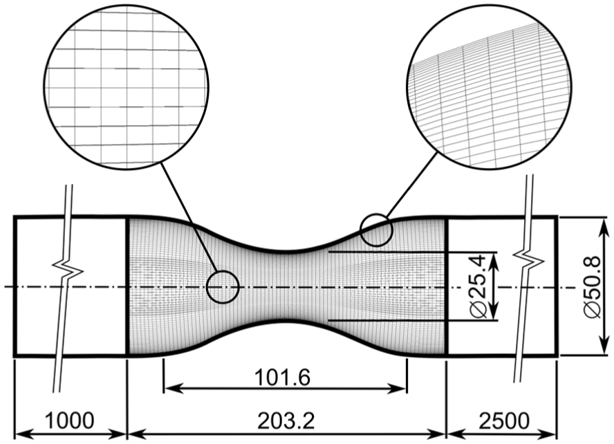
Details of the model geometry and its mesh.

The independence of the results on the computational mesh size was tested by simulations with four different mesh resolutions. The grid independence test was performed with one model based on RANS approach (standard low-Reynolds number k–ε model) and one LES model (wall-adapting local-eddy viscosity subgrid scale model), due to the wide variety of turbulence models used for the final comparison. The axial velocity profile along the stenosed tube centreline was monitored. The following mesh sizes were tested: 0.72, 2.01, 3.21 and 4.16 million cells. The result comparison (see Figure 2) showed that the differences in the profiles of the RANS approach were minimal, while the centreline profiles calculated using the LES model showed significant differences between the coarser and finer meshes. In the RANS case, all the meshes can be considered as independent while for the LES approach, only a solution performed on more than 3.21 million cells is independent on the mesh resolution. The computational time saving is an important parameter in a majority of industrial simulations, and the mesh resolution plays a big role in this field. However, this work focuses on the comparison of different modelling approaches, and for this purpose, it is necessary to keep identical conditions when possible. Therefore, a mesh consisting 3.21 million cells was chosen for the comparison of the turbulent models used in the article.

Figure 2.

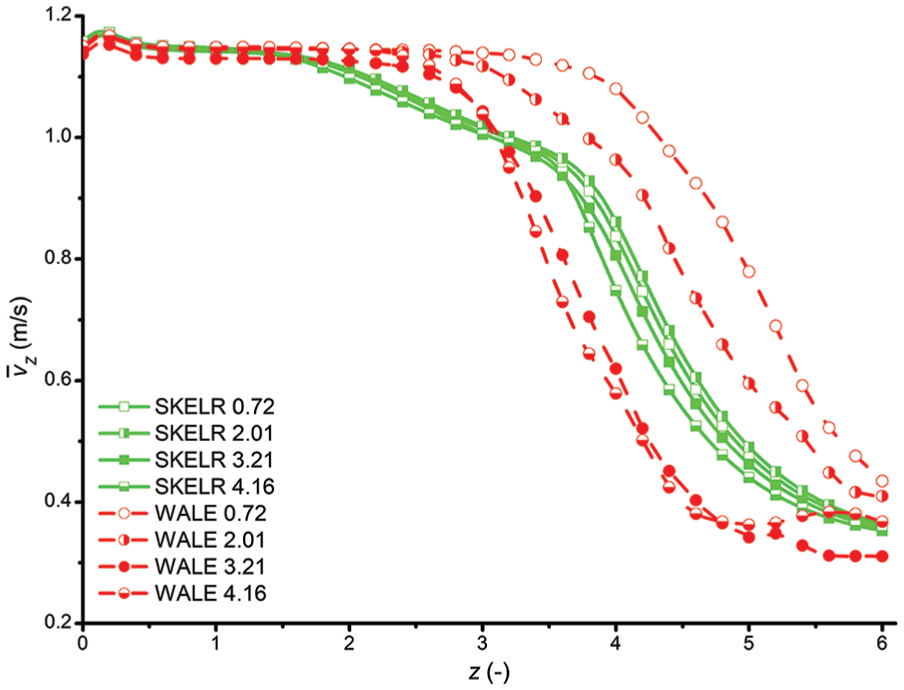
The grid independence test.

Flow simulations

In this study, the calculations were performed using the Star-CCM+ v.10.04 commercial solver. Experimentally measured values at Re = 2000 were considered for comparison. $Re = {\bar{v}}_{in} D ρ / μ$ , where ${\bar{v}}_{in}$ is the mean inlet velocity, D is the diameter of unconstricted tube, ρ is the density of the fluid, and μ is the dynamic viscosity of the fluid. Ahmed and Giddens³ specified that the 63% glycerol by weight at a temperature of 33°C was used as a fluid in their experiment. These parameters correspond to a fluid with dynamic viscosity of µ = 0.008 Pa s and density of ρ = 1156.5 kg/m³ according to Glycerine Producers Association.²⁵ Based on these values, the calculations of average inlet velocity yielded a value of ${\bar{v}}_{in} = 0.272 m / s$ . Since we shortened the original tube, a fully developed parabolic velocity profile with average velocity ${\bar{v}}_{in}$ was prescribed at our tube inlet instead of uniform values. Since the experimental flow rate corresponds to the laminar behaviour, it was decided to prescribe a low value of turbulence intensity (1%) at the inlet. According to Tan et al.,²³ moderately low values of turbulence intensity allowed to reasonably capture the experimental data. Also Cui,²⁶ who applied the LES–Smagorinsky model, achieved better results for lower prescribed values of turbulence intensity. The outlet boundary condition was prescribed as the pressure outlet with zero pressure resistance. Present calculations were performed with time step of t = 0.125 ms chosen to satisfy a Courant condition of C_f = 1.

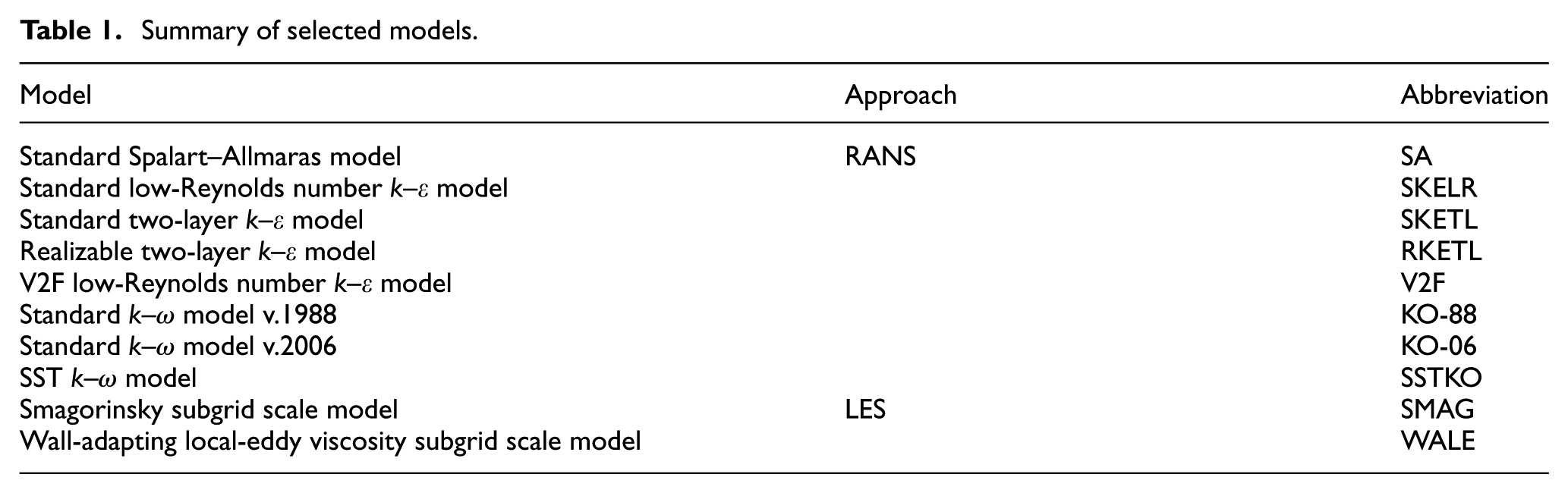
Temporal discretization was performed by the implicit unsteady algorithm with the second-order temporal discretization scheme. The convection term was, for all the RANS models, discretized using the second-order upwind scheme, while for the LES approach, a bounded central-differencing scheme was used. Turbulence was solved using 10 different models. Only those models that support complete resolving of the boundary layer taking low wall y⁺ approach into account were selected. Due to the comparison of a large number of heterogeneous approaches, all turbulent models and their constants were not modified but their default values set by the developer of the software were kept. The turbulence models considered in this study can be divided into four separate groups. The first group of turbulence models is represented by the standard Spalart and Allmaras²⁷ model (SA) which solves a single transport equation determining the turbulent viscosity; it was mainly developed for aerospace industry. This model was chosen to test its usability in the channel flow although it is not primarily designed to simulate similar cases. The second group contains the models with k–ε turbulence approach, which is generally considered as best for its robustness and accuracy of good resolving of free stream and complex recirculating flows. These models are standard low-Reynolds number k–ε model²⁸ (SKELR), standard two-layer k–ε model²⁹ (SKETL), realizable two-layer k–ε model³⁰ (RKETL) and V2F low-Reynolds number k–ε model³¹ (V2F). The third group is represented by models based on k–ω approach; they perform better than the k–ε models in the case of boundary layers, including the viscous-dominated region. Wilcox’s original standard k–ω model version from 1988³² (KO-88) and also its revised version from 2006³³ (KO-06) were used for comparison as well as the Menter’s modification of Wilcox’s model – SST k–ω model³⁴ (SSTKO), which combines benefits of k–ω approach in the near-wall region with good sensitivity of k–ε models in free stream. The last group is formed by a couple of models representing LES approach – Smagorinsky³⁵ subgrid scale model (SMAG) with Vandriest³⁶ damping function activated and wall-adapting local-eddy viscosity subgrid scale model³⁷ (WALE). SMAG and WALE constants were used with the default values pre-set by the programme (C_S = 0.1, C_W = 0.544). The complete list of models used and their abbreviations are mentioned in Table 1. All the calculations were performed for 3 s to ensure a fully developed flow, then selected variables were averaged for t = 2 s. Six cross sections were chosen for comparison purposes in accordance with the experiment. The positions of these cross sections can be seen in Figure 3 where z is the dimensionless axial coordinate measured from the throat of the constriction z = Z/D, where Z is the axial distance from the throat of the stenosis.

Table 1.

Summary of selected models.

Model	Approach	Abbreviation
Standard Spalart–Allmaras model	RANS	SA
Standard low-Reynolds number k–ε model		SKELR
Standard two-layer k–ε model		SKETL
Realizable two-layer k–ε model		RKETL
V2F low-Reynolds number k–ε model		V2F
Standard k–ω model v.1988		KO-88
Standard k–ω model v.2006		KO-06
SST k–ω model		SSTKO
Smagorinsky subgrid scale model	LES	SMAG
Wall-adapting local-eddy viscosity subgrid scale model		WALE

Figure 3.

The constricted tube with the positions of the cross sections used for comparisons with the experiment.

Components of velocities parallel to the axis of the constricted tube were monitored. The calculations were performed on eight cores of Intel Xeon E5-2690 processors which are contained in the computing cluster located at Brno University of Technology. The average run time for one variant of calculation was 100 h.

Particle deposition simulations

For selected turbulence models, a particle deposition using Lagrangian multiphase model was enabled. Particles with three different Stk (10⁻⁴, 10⁻³ and 10⁻²) were studied. These values of Stk correspond in the studied case of constricted tube with water–glycerine mixture as flowing fluid to spherical particles with density of ρ = 10,000 kg/m³ and sizes of 16, 52 and 164 μm. The corresponding diameters of aerosol particles with the same Stk, density of water (ρ = 1000 kg/m³), and suspended in air in the human trachea during light activity breathing would be 0.3, 1.0 and 3.3 μm, respectively.

For unsteady RANS models of turbulence, a turbulent dispersion model based on Gosman and Ioanides³⁸ enabled a more realistic simulation of the behaviour of particles. In all, 370,000 individual particles for each particle size were injected into the fluid through 31 release points during 0.3 s, and their tracking and deposition were performed for 3 s (see Figure 4). Particles were released into the domain at a distance of 0.2 m from the middle of the constriction.

Figure 4.

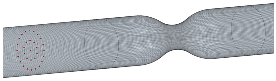
Detail of 31 release points for injection of the particles into the fluid.

Results

In this section, the results of our flow simulations in the constricted tube for Re_in = 2000 are compared with the experimental fluid velocity profiles measured by Ahmed and Giddens.³ Radial and axial velocity profiles are used to describe the differences between the models and the experiment.

Velocity profiles along the centreline

The mean axial velocity, computed for each turbulence model, was normalized by ${\bar{v}}_{in}$ according to Ahmed and Giddens³ and the profiles of this normalized mean axial velocity ${\bar{v}}_{Z}$ along the centreline of the tube in the neighbourhood of the axisymmetric constriction are shown in Figure 5 as a function of the dimensionless axial coordinate (see Figure 3). Differences between the centreline velocity predicted by the models and the experimentally measured value are added opposite to each of the models as seen in the legend in Figure 5. (The differences between the centreline velocity predicted by the models and the experimentally measured value were calculated as follows: The data from formerly published studies were digitized and transported into OriginPro 9 software (originLab, Northampton, MA, USA) as well as our model datasets. Then, the experimentally acquired values were subtracted as reference data from the respective model datasets. This procedure produced curves showing differences between the models and the experimental data as a function of the dimensionless distance z. To facilitate a quantitative comparison of various models, integration of the curves was performed in the range of z = (0–6), calculating the absolute area under the curve. These values were normalized by the area under the curve of the experimentally measured centreline and expressed in percents. Measurement errors can be expected in the range of units of percent, so for the deviations less than ∼6%, it does not make sense to rank them according to their reported deviations. The simulations showing deviation less than 10% can be qualified as well-matching models.)

Figure 5.

Comparison of computed axial velocity values along the centreline of the constricted tube with the experimental results of Ahmed and Giddens.³

Most of the models predict, in accordance with the experiment, a constant centreline velocity ${\bar{v}}_{z} ≅ 4.2 {\bar{v}}_{in}$ closely behind the throat at 0 < z ≤ 1. Only the SKETL and RKETL models feature a divergence from the experiment for all the inspected area.

Several models (SKELR, all the k–ω (KO-88, KO-06 and SSTKO) and the V2F model) feature a change in the trend from the constant velocity level to a moderate declination of the velocity with almost constant slope in the following portion of the tube. This feature could not be resolved in the experimental data points of Ahmed and Giddens³ due to their low spatial resolution, but it was found in other experiments³⁹ and numerical simulations.^26,40,41 This moderate declination ends when ${\bar{v}}_{z}$ drops below $3.6 \bar{v}$ . It suggests for the evolution of the shear layer of the separated flow in the post-stenotic section before the models predict the onset of turbulence and it is typical for laminar separated flows with a formation of recirculation zones.

All the models, except the KO-06 model, involve the transition from laminar to turbulent flow, which is indicated by a steep drop down of the centreline velocity with increasing z distance; however, each of the models provides a different breakpoint position. The experimental data evidence the onset of the transition at z ≅ 2.5. The SKETL, RKETL and SA models provide the laminar–turbulent transition unrealistically, just behind the constriction end at z = 0.2–1, and the turbulent flow develops very early; these models clearly fail to treat the expanded flow. The SKELR, SMAG and WALE models are consistent with the experimentally observed character of the transition; their progress to turbulence is similar and only slightly steeper than the experiment shows. While the WALE model matches best with the experimental data points in the transitional region (2.5 < z < 5), the SKELR model treats best the past flow for z > 5, where the other two trusty models rather underpredict the centreline velocity. The rest of the models places the transition origin to z = 4.5, 5 and 5.75 applying for V2F, SSTKO and KO-88 models, respectively.

Radial velocity profiles

A more detailed result of comparisons is given by the radial profiles of the mean axial velocity at the axial stations z = 0, 1, 2.5, 4, 5 and 6 downstream of the stenosis throat (Figure 6). The radial profiles are shown as a function of the dimensionless radial coordinate r = r_c/R where r_c is radial coordinate measured from the centreline of the tube and R is the actually inspected tube radius and the points 0 and 1 stand for the tube axis and the wall position, respectively. The axial symmetry of the mean radial profiles was considered and only half radial profiles of the axial velocity are shown for the comparison of the simulated and measured data in accordance with the practice introduced by Ahmed and Giddens.³

Figure 6.

Comparison of computed radial profiles of axial velocity in the constricted tube with the experimental results of Ahmed and Giddens.³

All the RANS models, except the SA model, predict the flow to be radially symmetrical, and also the LES models feature only a very weak asymmetry of the radial velocity profile (see Appendix 2, Figure 11). The SA model demonstrates a strong asymmetry of the post-stenotic flow by causing the jet to deflect towards the bottom wall in the downstream region as shown in Appendix 2, Figure 11. This asymmetry in the SA model explains the apparent deviation of its radial velocity profile in comparison with the other results in Figure 6.

The existence of flow asymmetry in the axisymmetric stenosis was manifested by several authors. Mallinger and Drikakis⁴² revealed highly asymmetric flow downstream of the three-dimensional axisymmetric stenosis. Sherwin and Blackburn⁴³ found a Coanda-type wall attachment of the steady flow in a straight tube with a smooth axisymmetric constriction due to a small perturbation added to the base flow. The flow through axisymmetric and eccentric stenoses models was studied in detail by Varghese et al.⁴⁴

The graphs in Figure 6 illustrate a qualitatively different character of the flow in the consequent z positions in the tube as well as the significant differences among the models. All the models predict almost identical flat flow profiles at the throat (z = 0); their results qualitatively correspond to the experimental data, but the velocity values are almost 10% larger than the experimental ones. This discrepancy is addressed below.

The experiment at the station z = 1 shows that the jet-core with the original velocity ${\bar{v}}_{z} ≅ 4.2 {\bar{v}}_{in}$ sharply turns into a stagnant zone with zero velocity values that spans in 0.6 < r < 1. This feature was well approximated by all the models, except SA, SKETL and RKETL.

The jet-core reduces its cross section with increasing flow distance; it is seen at z = 2.5 that the velocity changes between the core and the flow separation zone become more gradual and the flow recirculation occurs near the wall. The experimental flow profile is still well represented by most of the models but the differences among them became evident. The last three stations (z = 4, 5, 6) show no presence of the jet but a gradual development of the flat-turbulent-like profile.

The experiment documents that the near-wall zone, where the flow separation and recirculation occur, begins immediately downstream of the throat and continues to the distance of three diameters downstream. The recirculation phenomena were well captured by most of the models at z = 2.5, while the SMAG and WALE models overpredicted its intensity and the SA, SKETL and RKETL models failed to treat it at all. The KO-88, SSTKO and V2F models predict the end of the recirculation zone at z ≅ 4; therefore, they overpredict the length of the recirculation region, and the KO-06 model places the end of the recirculation region even to z ≅ 5. The SKELR model well agrees with the experiment in terms of the intensity and positioning of the recirculation zone.

After that the transition to the turbulent profile can be seen. The SA and SKETL models predict a gradual transition of the velocity profile, reaching the fully developed turbulent profile at z = 4 already; this development is similar for the SMAG, WALE and RKETL models at z = 5, and for SKELR at z = 6. The SSTKO model approaches the transient profile of the experiment at z = 6, while the KO-88, KO-06 and V2F models show more deformed profiles. The best qualitative and quantitative match with the experiments over the six stations was found for the SKELR, SMAG and WALE models consistently with the findings in Figure 5.

The simulated flow fields behind the constriction are detailed in Appendix 2, Figure 11, for all the tested models.

To summarize, it was shown that different turbulence models estimate the flow character with different accuracy and that even the flow through such a trivial geometrical shape as the stenosed smooth tube is very intricated for the present turbulence models. Three models perform comparatively well in terms of the mean axial velocity, in the inspected area of 0 < z ≤ 6 (SKELR, SMAG and WALE) with error between 5.5% and 7.1%. The other considered models did not capture the flow faithfully showing the error between 14% and 32%.

Turbulence along the centreline

The turbulence and its longitudinal development were evaluated on the basis of the axial velocity fluctuations normalized by the mean inlet velocity – see Figure 7. The differences between the LES models and experiment are of similar magnitude to those reported by Tan et al.²³ The velocity fluctuations were for RANS approach based on assumption of isotropic turbulence and calculated as $u' = \sqrt{2 \cdot k / 3}$ .

Figure 7.

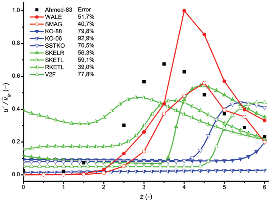
Comparison of the computed axial disturbance velocity profiles along the centreline of the constricted tube with the experimental results of Ahmed and Giddens.³

As can be seen, some models even failed to predict the position of the maximum within the solution domain – namely, the KO-06 and KO-88 models. The KO-88 shows a tendency to rise to its maximum of the turbulent fluctuations towards the end of the solution domain, but the KO-06 completely fails. The model is also very sensitive to inlet boundary conditions, which is a disadvantage not seen, for example, in k–ε. However, we kept the inlet conditions with all models identical. The other models show approximately comparable values of the maxima of the turbulent fluctuations, but the maxima themselves are shifted either upstream or downstream of the experimental maximum. As for the position of the maxima of the fluctuations, the best agreement can be seen with RKETL model with a lower maximum as compared with the experiments. This model subdivides the whole solution domain into a viscosity-affected region and a fully turbulent region. The distinction between the two regions is determined by a wall-distance-based turbulent Reynolds number defined with k value and the normal distance from the wall. In the near-wall region, only k equation is solved, and the length scale is computed.

Higher values of the maxima are predicted by SMAG and SKELR model. The maxima given by both models are identical, but the SKELR shows a delayed and a more rapid increase in the fluctuations and a slower decrease. The SSTKO and V2F models show a similar course with the maximum shifted towards the end of the solution domain, that is, considerably delayed rise. The highest value of the maximum is produced with the WALE model with the peak position close to the experimental value but the absolute maximum value is much larger than for all other models and experiments. We omitted the SA model in the graphs. This is a one-eq1 turbulence model developed specifically for aerodynamic flows such as transonic flow over airfoils with only a single equation for turbulence and with a strong limitation in shear flows and separation. In other words, the model is unable to correctly predict separation; for example, it predicts the flow attached long after it has separated in reality.

SST

It is claimed that its performance is not very different from the RKETL. The model has gained this popularity based on its ability to predict separation and reattachment better when compared to k–ε and the standard k–ω. However, as can be seen from the graph, this model shifts the maximum too far from the experimentally obtained value in contrast to RKETL. This is very probably given by the fact that the model has issues predicting turbulence levels and complex internal flows. The issue is also the fact that the blending function crossover location (blending between k–ε in the far field and k–ω near the target geometry) is arbitrary and could obscure some critical feature of the turbulence.

From the above, we can conclude that the best match as for the course of the velocity fluctuations and their maxima (absolute values and positions) compared with experiments is predicted by two RANS models, namely RKETL, which predicts the best maximum position, and SKELR, which predicts the best maximum value. SMAG predicts the best maximum value identically with SKELR.

The fluctuations of the secondary components (the fluctuations in the radial and circumferential directions) are shown in Figure 8 for the LES models. Their values are identical to the axial component for the RANS models due to their assumption of the isotropic turbulence.

Figure 8.

Comparison of computed secondary disturbance velocity profiles along the centreline of the constricted tube with the experimental results of Ahmed and Giddens.³

The differences between the velocity fluctuations predicted by the LES models (SMAG and WALE) and the experimentally measured values were calculated in the same way as the differences between the predicted and measured mean velocities.

The experiment indicates approximately 20% difference between the axial and secondary fluctuations while the SMAG and WALE model predict approximately 40% and 75% difference, respectively. Although it is generally expected that the LES models are accurate in the core region, the differences in axial fluctuation components for the two (WALE and SMAG) models for identical boundary conditions prove that even LES does not guarantee sufficiently realistic results.

Also, the experimentally measured values of the velocity fluctuations must be taken with care; their uncertainty is naturally much higher than that for the mean velocity due to the experimental noise (see ‘The accuracy of the results of Ahmed and Giddens’ section).

Comparison with published simulations

The experimental data of Ahmed and Giddens^2,3 for the stenosed flow case were used by many authors to validate their numerical models. We have used the published data that allowed matching with our results (the same stenosed geometry with 75% constriction, Re = 2000, data containing the mean axial velocity profiles) to supplement our model set and comparison of their prediction abilities.

Zhang et al.⁴⁵ adapted the LRN k–ω model of Wilcox³² (denoted thereafter as Zhang-02-LRKO) for internal flow studies in a user-enhanced commercial finite-volume based programme CFX4.4. Later, Zhang and Kleinstreuer⁴⁰ considered LRN k–ε (Zhang-03-LRKE), RNG k–ε (the axial profiles of the velocity for the RNG k–ε model were missing in the article, but the radial velocity profiles together with the discussion showed that this model failed to treat the modelled flow regimes), LRN k–ω (Zhang-03-LRKO) and Menter k–ω (Zhang-03-SSTKO) models, using the same programme on the stenosed geometry with 560,000 cells. This group⁴¹ finally compared the performances of LES WALE (Zhang-11-WALE) and three turbulence models, including standard k–ω (Zhang-11-KO), LRN k–ω (it is the same model as the LRN k–ω model presented in Zhang and Kleinstreuer⁴¹ and Zhang and Kleinstreuer⁴⁰) and SST transitional (Zhang-11-SSTKO) models with hexahedral mesh (1,140,480 elements).

Luo et al.⁴⁶ employed three numerical methods, laminar flow, k–ε model and LES models (Luo-04-LAM, Luo-04-KE and Luo-04-LES, respectively), and a grid with 227,981 cells using the commercial CFD package, Fluent 5.3.

Cui²⁶ used LES and adopted both the SMAG³⁵ and dynamic SMAG^47,48 where 2% (Cui-12-SMAG2) and 4% (Cui-12-SMAG4) inlet velocity fluctuations were adopted. This author used 2,731,820 grid nodes and a hexagonal mesh in the software platform of OpenFOAM^® 1.5. A summary of these published models is given in Table 2.

Table 2.

Summary of published models used for comparison.

Source	Approach	Solver	Abbreviation
Cui²⁶	Smagorinsky subgrid scale model	OpenFOAM^® 1.5	Cui-12-SMAG2
Cui²⁶	Smagorinsky subgrid scale model	OpenFOAM^® 1.5	Cui-12-SMAG4
Luo et al.⁴⁶	RNG-based subgrid scale model	Fluent 5	Luo-04-LES
Luo et al.⁴⁶	k–ε model	Fluent 5	Luo-04-KE
Luo et al.⁴⁶	Laminar flow	Fluent 5	Luo-04-LAM
Zhang et al.⁴⁵	Low-Reynolds number k–ω model	CFX 4.4	Zhang-02-LRKO
Zhang and Kleinstreuer⁴⁰	Low-Reynolds number k–ε model	CFX 4.4	Zhang-03-LRKE
Zhang and Kleinstreuer⁴⁰	Menter k–ω model	CFX 4.4	Zhang-03-SSTKO
Zhang and Kleinstreuer⁴¹	Standard k–ω model	ANSYS CFX	Zhang-11-KO
Zhang and Kleinstreuer⁴¹	SST transitional model	ANSYS CFX	Zhang-11-SSTKO
Zhang and Kleinstreuer⁴¹	Wall-adapted local eddy-viscosity model	ANSYS CFX	Zhang-11-WALE

The profiles of the normalized mean axial velocity along the centreline of the tube are presented for these selected published results along with our prospective models (the SKELR, SMAG and WALE) in Figure 9 in the same way as it was in Figure 5.

Figure 9.

Comparison of the computed axial velocity along the centreline of the constricted tube with the published simulations^{26,40,41,45,46} and experimental results.³

Clearly, several published models failed to mimic the experimental velocity profile. The Zhang-03-LRKE, Luo-04-KE and Luo-04-LAM models differ from the experiments by more than 26%, and even the Luo-04-LES produces a 14% difference.

The rest of the models predict well the s-shaped course of the axial profile of the centreline velocity with a similar steep transition from the maximum velocity closely behind the throat (z = 0) to the low velocity at the end of the inspected area (z = 6). The maximum and minimum velocity values vary model to model, and mainly, the z position of the transition from the laminar to turbulent flow apparently differs. Most of the models predict earlier transition than the experiment while all our models and Zhang-11-WALE adversely.

Our SKELR model with 7.1% difference is comparably as good as the Zhang-02-LRKO, Zhang-11-SSTKO and Zhang-03-SSTKO models that match the experiments with 7.8%–9.7% error. The best performance was provided by the LES models of Cui,²⁶ with 3.5% and 4.6% difference, and Zhang and Kleinstreuer⁴¹ (5.5% difference), followed by our WALE and SMAG simulations with 5.5% and 6.5% difference, respectively.

Results of simulated deposition of particles

A deposition rate of particles was expressed as a deposition fraction in successive cylindrical surface areas. The deposition fraction is a ratio of the number of deposited particles in the examined region to the total number of particles injected into the tube. Deposition fractions calculated from the results of three models (SKELR, SMAG and WALE) are summarized in Figure 10. The constricted tube was divided into 14 cylindrical areas. The first area, called ‘Upstream’, is the surface of tube from the injection point (z = −2) to the throat of the constriction (z = 0). It is followed by 12 equidistant areas with length of 0.5 D. They are represented by their upper bound (e.g. the first area of the cylinder from the throat of the constriction to z = 0.5 is represented by 0.5) in Figure 5. The particles deposited further downstream after z = 6 are represented by the term ‘Downstream’, and the particles that penetrated through the whole tube are represented by the term ‘Non-depositing’.

Figure 10.

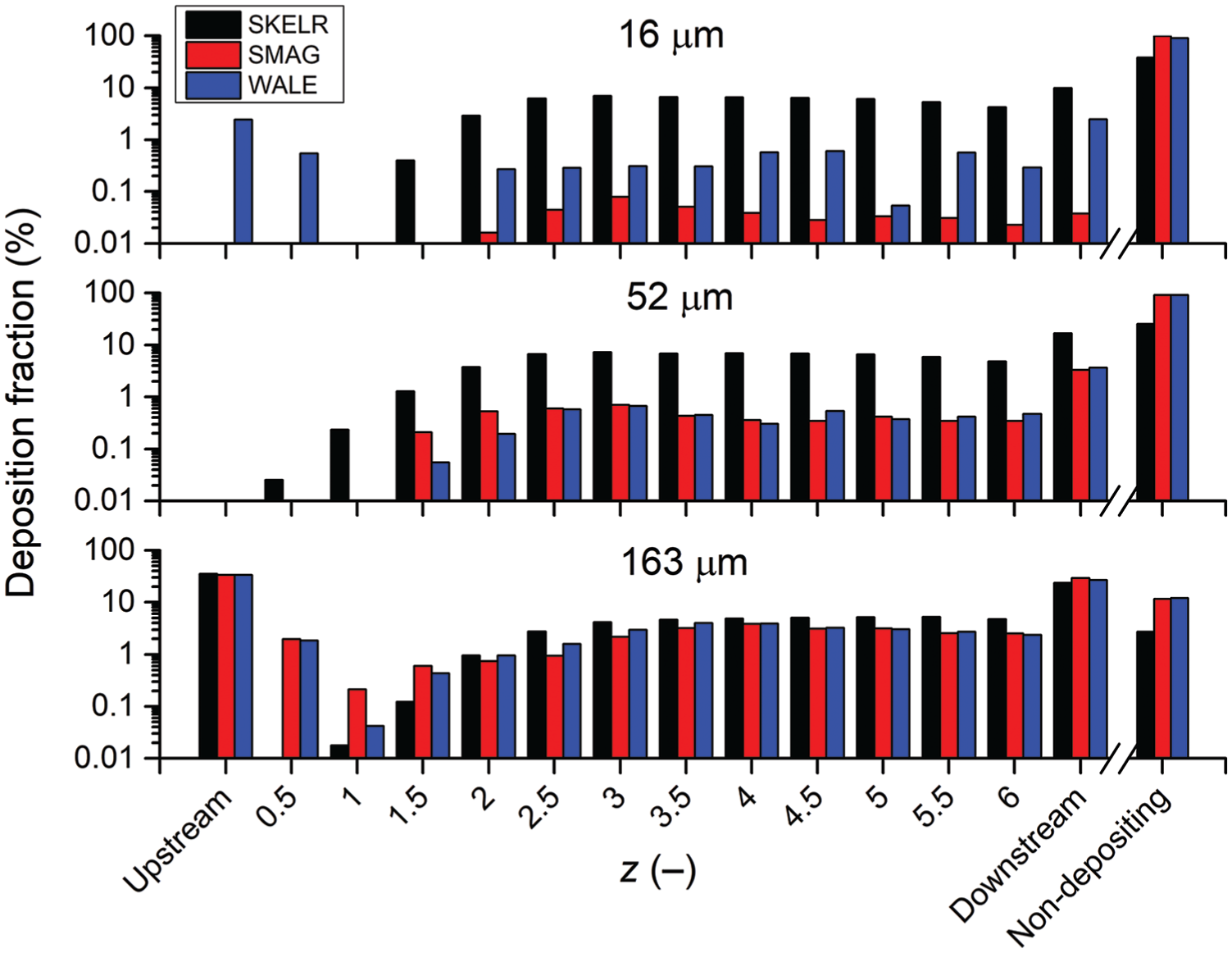
Deposition fraction of 16, 52 and 163 μm particles calculated by SKELR, SMAG and WALE.

A comparison of deposition fraction in Figure 10 clearly shows that there were substantial differences among the models, especially for the case of the smallest 16 μm particles. The SKELR model predicted no deposition upstream of the constriction, and a significantly larger deposition compared to both LES models in the tube downstream. Based on the results in Figure 10, there were large differences even between the two LES models. Only the WALE model predicted any deposition upstream. Both LES models gave a similar prediction of deposition for 52 and 163 μm particles. SKELR predicted a larger deposition in all zones for 52 μm particles. For 163 μm particles, there were almost no deposited particles predicted by SKELR in the zone from z = 0 to 1. In general, the larger the particles, the smaller the differences among the models.

Discussion

The flow character

The structure and development of the flow past the stenosis depends on the stenotic geometry (stenosis degree, shape and eccentricity) and flow conditions (steady/unsteady, Reynolds number). This case of steady flow cosine stenosis (cosine contour) features a fully turbulent post-stenotic flow at Re = 2000, according to the results from Ahmed and Giddens.³ Solzbach et al.⁴⁹ showed that, for the 75% constriction, the typical Re_c = 600 (critical Re). However, the Re_c varied between 500 and ca. 1100 depending on the stenotic geometry. According to the map of the flow stability given by Griffith et al.,⁵⁰ the flow in our case is absolutely unstable.

The post-stenotic flow is characterized by the core jet and a flow separation region, which features ‘an intricate pattern of shed vortices that roll on top of each other and merge in the expansion zone distal to the stenosis throat’ as described by Bluestein et al.⁵¹ for Re = 1550. Generally, for Re > 1000, Bluestein et al.⁵¹ observed that ‘…the site of vortex initiation is very near the stenosis throat at the point of flow separation … the dissipates before reaching the end of the stenosis region’. Cui²⁶ reports that ‘After this relatively steady period, the velocity decreases quickly because the flow transits from laminar to turbulent coupled with large-scale lateral momentum transfer. In addition, it is described that the flow transition occurs in the region 1 < z < 4³’.

The accuracy of the results of Ahmed and Giddens

The experimental data contain uncertainties of several types. These uncertainties can limit the validation possibilities.³

The measurement method itself has a limited precision and resolution. However, Ahmed and Giddens did not report experimental uncertainties of their data obtained from their laser Doppler anemometry (LDA) measurements. We can expect these to be in lower units of percent.²⁰

The boundary conditions (inlet turbulence intensity, flow velocity, fluid viscosity among others) can be significant as well. Varghese et al.⁴⁴ studied steady and pulsatile flow through a 75% constricted tube using direct numerical simulations (DNS). According to their results, a laminar flow downstream of an axisymmetric stenosis appeared even at the inlet Re = 1000, which greatly differs from the LDA results of Ahmed and Giddens.³ Varghese et al.⁴⁴ suggested these differences to the upstream noise (i.e. flow fluctuations) in the experimental set-up.

The imperfections of the model geometry (asymmetry, fabrication tolerances for size and shape) and wall roughness is another issue. For example, Griffith et al.⁵⁰ suggested the presence of a turbulent breakdown of the flow triggered by experimental noise which was able to explain the discrepancy between the turbulent experimentally found post-stenotic flow and the laminar flow from their CFD simulations. Varghese et al.⁴⁴ showed that the stenosis eccentricity may cause transition to turbulent flow at Re = 1000.

Zhang and Kleinstreuer⁴¹ showed that the measured data sets of Ahmed and Giddens³ do not accurately reflect mass conservation and uncertainties exist in regions of large velocity changes. ‘However, the measured velocities are apparently lower than their expected values at the throat (z = 0) based on mass balance calculations, which can be attributed to experimental uncertainties’. ‘The experimental profiles indicate that the flow reattaches to the wall between z = 4 and 6, which may also imply that the flow does not remain completely laminar because of upstream noise and possible geometric perturbation (e.g. stenosis eccentricity)’.⁴¹

Discussion on the flow models

The results summarized in Figures 5 –9 allowed to assess the abilities of the LES and the RANS turbulence models to treat the stenosed flow case.

The wrong performance of the SA model in the channel flow is not surprising as it was designed specifically for aerodynamic flows; it is not calibrated for general industrial flows and produces relatively large errors for some free shear flows.

The laminar flow model of Luo et al.,⁴⁶ Luo-04-LAM, obviously underestimated the turbulent energy dissipation downstream of the stenosis.

The family of the different k–ε approaches features the widest scatter over the experimental results. Even the two standard low-Reynolds number k–ε models used (Zhang-03-LRKE and SKELR) performed differently; while SKELR approximated well the experimental measurement and registered the laminar–turbulent transition, the Zhang-03-LRKE failed to show it at all. The low-Reynolds number model included in Star-CCM+ is a version produced by Lien et al.²⁸ and its coefficients are identical with the standard k–ε model but provide more damping functions. These functions are applied in the viscous-affected regions near walls. The Luo-04-KE assumes too much energy dissipation and fails to correctly predict the tendency of the flow evolution. The SKETL and RKETL models provide the laminar–turbulent transition unrealistically early but perform well in the developed area. The RKETL is more precise than the SKETL model as it benefits from its improved predicting abilities to resolve the flows involving separation and recirculation and to capture the complex flows. The V2F model, though designed to handle the near-wall turbulence effects more accurately, failed in this case to show its quality as the transition was modelled as too late. These findings suggest that the choice and setting of the k–ε model can drastically affect its success in such transient flow cases.

The k–ω models in comparison with the k–ε models benefit from their better ability to treat the wall effects present within this flow case. While the Zhang-11-KO model somehow overpredicts flow instabilities and essentially follows the experimental data points, both our k–ω models (KO-88 and KO-06) fail to treat the low-Reynolds number flows in laminar-to-transitional regimes. The original k–ω model (KO-88) outperformed the version with revised set of model coefficients (KO-06), which suggests that further validations of this successor for the complex flows are needed and it should be set with caution.

A comparison of our and published results demonstrates that it is possible to set the k–ω model parameters to capture the stenosed flow. A good performance of the Zhang-11-KO model results from the coefficient modifications; the particular coefficients given in the paper of Zhang and Kleinstreuer⁴⁰ differ from those of our models (default settings) in a number of values.

Our SSTKO model (see Figures 5 and 6) largely underestimates the turbulence behaviour (dissipation) as it approaches the transient profile of the experiment as far as where z = 6 and it overpredicts the length of the recirculation region. On the contrary, the two SSTKO models of the Zhang’s group (Zhang-03-SSTKO and Zhang-11-SSTKO) behave quite differently (see Figure 9). These models overemphasize the flow instabilities after the throat and perform relatively poorly in the region of shear layer development and recirculating flows (area between approximately z = 1.5 and 5), while their prediction of mean velocity profiles in the region after the onset of turbulence (z > 5) is consistent with the experiments. Therefore, all the SSTKO models fail to capture the velocity profile in the transitional regime and predict the onset of turbulence in the post-stenotic expanded region where a large-scale momentum transfer applies.⁴⁰

The Zhang-02-LRKO model (see Figure 9) predicts a weaker post-stenotic turbulence when compared to the laboratory measurements but it can model the post-stenotic flow including the evolution of the shear layer, the recirculation region, and the onset of turbulence. Its consistency with the experimental data points overcomes all the standard and SSTKO models.

The results of all the simulations based on the Smagorinsky approach agree well with the experimental results. In particular, in the transitional regime, their performance is better than that of other models; they can resolve the evolution of the shear layer and recirculation zone. The differences between the results of Smagorinsky models by Cui²⁶ and our SMAG simulation can be partially explained by different inlet turbulence settings (2%, 4% and 1%, respectively), but the difference between the Cui’s case for 2% inlet turbulence and our result, which is much larger than between both the Cui’s models, suggests that also some other simulation variables were set differently. Cui set the Smagorinsky constant to C_s = 0.167 in the Smagorinsky subgrid scale model without any reasoning. The user guide⁵² for the Star-CCM+ solver declares that the typical values of C_s reported in the literature span from 0.07 for flows in channels to 0.165 for homogeneous isotropic decaying turbulence. The default value of C_s = 0.1, used in our case, is a compromise between these extremes.

The relatively large 14% discrepancy between the Luo-04-LES results and the experiment can be explained by the inlet turbulence settings in simulations of Luo et al.⁴⁶ He used the turbulent intensity of 6.18% which he claimed to be the same as in the experiment of Ahmed and Giddens;³ however, we did not find such a high value in the reported paper. Luo et al.⁴⁶ himself explained the limited accuracy of his results by the grid size used.

Both LES WALE models (our WALE and Zhang-11-WALE) show unsurprisingly similar trends and they very well capture the flow characteristics in the inspected area behind the stenosis and, namely, in the transitional region (2.5 < z < 5), including the flow structures and transition to turbulent flow.

Discussion over the simulated deposition of particles

There are several mechanisms that cause a deposition of particles in a straight tube with constriction including gravitational settling, diffusional deposition, turbulent inertial deposition, inertial deposition at flow constriction and interception.⁵³

The gravitational mechanism can be described using a balance of internal and external forces acting on the particle, specifically the buoyant Archimedes force, drag force, and gravitational force. A constant settling velocity establishes after a very short interval, usually fractions of second.⁵⁴ A solution of the balance of forces shows that the particle settling velocity v_s is a function of drag coefficient C_d, which depends on the settling Reynolds number Re_s = v_s·d_p·ρ_f/µ. There are four different regimes of settling, and for each of them, a specific expression of C_d must be used. The first regime is called Stokes region and is defined by Re_s < 0.2. Allen (sometimes called transient) region is specified by 0.2 < Re_s < 10³. Higher flows then fall either in Newton (10³ < Re < 1.5 × 10⁵) or supercritical region (Re > 1.5 × 10⁵). The differences in C_d within the Stokes and Allen regions are in approximately three orders of magnitude; hence, the calculated v_s is extremely sensitive to appropriate determination of the settling regime.

Whether the particle settles or not depends on its residence time, that, in order to deposit, must be larger than the settling time. The settling time in non-stirred environment with pure gravitational settling in horizontal tube can be estimated as an altitude of the particle h divided by the v_s. Rough estimate of particles deposited by gravitational settling can be made on the basis of initial particle axial velocity equal to the surface average velocity of the flow, and the altitude of the particle. Calculation for a particle in the middle vertical plane of the tube shows that particles of diameter 16, 52, and 163 μm deposit if their initial altitude is smaller than 0.4%, 4.7%, and 47% of the tube diameter, respectively.

It should be noted that categorization to the settling regime is not trivial, as the Re_s only takes into account the velocity of the particle (which is, however, unknown at the beginning of the calculation). Yet, small particles are being stirred by Brownian motion, and even some larger particles are carried by eddies in the case of turbulent flows. These disturbances shift the real regime to the higher flow regions. Moreover, the simultaneous effect of various deposition mechanisms may increase or decrease the total deposition depending on the boundary conditions.

The mechanism of diffusional deposition is significant only for small particles (in the airways, the particles with diameter smaller than 1 μm). Particles influenced by Brownian motion diffuse from high concentration to low concentration region, while the wall acts as a sink.⁵³ In the present work, a contribution of this mechanism to the total deposition is negligible, as even the smallest 16 μm particles are too huge to be transported by Brownian motion in high numbers. It is worth noting that particle displacements due to turbulent diffusion dominate over Brownian displacements even for small particles, except the near-wall region.⁵⁵

Turbulent inertial deposition may exist in three different regimes. The first one combines turbulent mixing in the central zone and the Brownian diffusion through the laminar sublayer to the wall. It only applies to small particles. The second one works in turbulent diffusion-eddy impaction regime and applies to larger particles with sufficient inertia. In this regime, the deposition increases with increasing inertia.⁵³ The third regime applies to even larger particles whose trajectories are less affected by turbulent disturbances and the actual deposition decreases with increasing particle diameter. The theory describing all three regimes by Eulerian approach was published by Guha.⁵⁶ The Lagrangian approach was described by Chen and Ahmadi.⁵⁷ A governing factor for turbulent inertial deposition is the particle relaxation time,⁵⁷ which can be described as the time the particle needs to react on the change of direction of the flow. The dependence of particle deposition on the relaxation time follows the V-shape curve. Also, according to Lee and Gieseke,⁵⁸ the flow Reynolds number has to be taken into account in Brownian and turbulent diffusion-eddy impaction regime. Hence, this deposition mechanism is also extremely sensitive to the correct solution of laminar–turbulent transition prediction in CFD.

The inertial deposition in the flow constriction can be predicted using Stk. As in our case, the Stk was below 10⁻² for all cases; we can assume that this mechanism was negligible. Similarly, interception applies mostly for the cases where the size of particles approaches the size of a tube as this mechanism applies for particles whose centre of gravity follows the streamline around the obstacle or wall; however, the surface of the particle touches the wall and causes a collision. Therefore, in our case, this mechanism has minor effect on total deposition.

Based on the above-mentioned analysis, we can speculate that the differences among the SKELR, SMAG and WALE models were caused by different predicted levels of turbulent dispersion, which mostly influences the turbulent inertial deposition. While, Gosman and Ioanides’³⁸ turbulent dispersion model was applied for SKELR, both LES models calculate the velocity fluctuations directly, and hence, they can be considered more appropriate for predicting the deposition. The conjecture that turbulent dispersion is responsible for the differences among models is supported by the fact that the largest differences were found for the smallest particles. For larger particles with higher inertia, which are not easily diverted from their trajectories by turbulence, the differences were small. As there is no experimental data on particle deposition in the Ahmed and Giddens geometry, it is difficult to judge which model performed best. Nonetheless, the results clearly showed that even the models which predict the flow field closely give different results regarding particle deposition. Therefore, experimental validation of numerically simulated deposition is highly recommended.

Conclusion

Several RANS and LES turbulence models were used to simulate the stenosed flow in accordance with the published experimental case of Ahmed and Giddens.³ The performance of these models was qualitatively and quantitatively compared with the experimental results and with various published flow models.

Three models in our flow simulations performed comparatively well in terms of the mean axial velocity. These are, namely, the SKELR and two LESs with SMAG and WALE subgrid scale models with 7.1%, 5.5% and 6.5% difference from the reference experimental data, respectively, while the other models considered did not capture the flow faithfully. The best performance was provided by the two published LES models of Cui²⁶ and Zhang and Kleinstreuer⁴¹ with 3.5%, 4.6% and 5.5% difference, respectively.

The comparison of the results from different numerical models shows that several models adequately predict the flow field transition from laminar to turbulent. It was shown that even the LES approach does not guarantee trustful results, and a rigorous validation of the simulations is a must. On the contrary, a properly selected RANS (SKELR) model can also perform well, and its application is justified by the advantage of time savings. The optimal selection of the model depends on the taskmaster requirements – if quality and precision have the highest priority, the WALE model (Cui-12-SMAG4) performs best. If the result swiftness is demanded, then SKELR is the choice with an acceptable loss of precision.

Our and published flow simulation results showed that different turbulence models estimate the flow character with different accuracy. Even the flow through a simple stenosed smooth tube is a very intricated problem for the present CFD models. Modelling of transient flows is more challenging than fully turbulent flows. Some of the models could perform better in higher turbulent regimes. In order to obtain reliable results, numerical models need to be validated for the same geometry and similar flow regime. And well-prescribed boundary condition, namely, the inlet turbulence, is crucial as well.

As the deposition of particles is of great importance in many applications of flow through constricted tubes, the ability to predict the deposition rates was tested using the models which faithfully predicted the flow features. It has been demonstrated that the correct solution of velocity field and laminar–turbulent transition is not sufficient condition for the correct prediction of deposition of particles. Modelling of turbulent dispersion appears as a crucial phenomenon that influences especially the turbulent inertial deposition. Its effect decreases with increasing size of particles. All models agreed well for large particles where gravitational settling dominates.

This study demonstrated that it is not sufficient to validate solely the flow, but particle tracking algorithms must be validated as some models mimic the flow accurately, but do not perform well regarding the deposition.

Footnotes

Appendix 1

Appendix 2

Handling Editor: Takahiro Tsukahara

Declaration of conflicting interests

The author(s) declared no potential conflicts of interest with respect to the research, authorship, and/or publication of this article.

Funding

The author(s) disclosed receipt of the following financial support for the research, authorship, and/or publication of this article: This work was financially supported from the project of the Czech Science Foundation GA18-25618S, from the project of the Czech national programme INTER-COST, LTC17087 as a part of the COST Action SimInhale MP1404, the project of the Brno university of technology FSI-S-17-4444 and the project “Computer Simulations for Effective Low-Emission Energy” funded as project No. CZ.02.1.01/0.0/0.0/16_026/0008392 by Operational Programme Research, Development and Education, Priority axis 1: Strengthening capacity for high-quality research. The financial support is gratefully acknowledged.

ORCID iDs

Jakub Elcner

Frantisek Lizal

Jan Jedelsky

References

Ahmed

Giddens

DP.

Pulsatile poststenotic flow studies with laser Doppler anemometry. J Biomech 1984; 17: 695–705.

Ahmed

Giddens

DP.

Flow disturbance measurements through a constricted tube at moderate Reynolds-numbers. J Biomech 1983; 16: 955–963.

Ahmed

Giddens

DP.

Velocity-measurements in steady flow through axisymmetric stenoses at moderate Reynolds-numbers. J Biomech 1983; 16: 505–507.

Elcner

Lizal

Jedelsky

et al . Numerical investigation of inspiratory airflow in a realistic model of the human tracheobronchial airways and a comparison with experimental results. Biomech Model Mechanobiol 2015; 15: 447–469.

Jedelsky

Lizal

Jicha

Characteristics of turbulent particle transport in human airways under steady and cyclic flows. Int J Heat Fluid Flow 2012; 35: 84–92.

Lizal

Belka

Adam

et al . A method for in vitro regional aerosol deposition measurement in a model of the human tracheobronchial tree by the positron emission tomography. Proc IMechE, Part H: J Engineering in Medicine 2015; 229: 750–757.

Belka

Lízal

Jedelský

et al . Application of image analysis method to detection and counting of glass fibers from filter samples. Aerosol Sci Tech 2016; 50: 353–362.

Jókay

Farkas

Füri

et al . Computer modeling of airway deposition distribution of Foster® NEXThaler® and Seretide® Diskus® dry powder combination drugs. Eur J Pharmaceut Sci 2016; 88: 210–218.

Farkas

Jokay

Furi

et al . Computer modelling as a tool in characterization and optimization of aerosol drug delivery. Aerosol Air Qual Res 2015; 15: 2466–2474.

10.

Vinchurkar

De Backer

Vos

et al . A case series on lung deposition analysis of inhaled medication using functional imaging based computational fluid dynamics in asthmatic patients: effect of upper airway morphology and comparison with in vivo data. Inhalat Toxicol 2012; 24: 81–88.

11.

Housman

Innovative tests for patient-tailored treatments: demonstrating value in the age of personalized medicine. Pers Med 2011; 8: 183–189.

12.

Jameson

Longo

DL.

Precision medicine – personalized, problematic, and promising. N Engl J Med 2015; 372: 2229–2234.

13.

Agusti

Bel

Thomas

et al . Treatable traits: toward precision medicine of chronic airway diseases. Eur Respirat J 2016; 47: 410–419.

14.

Elkins

Taylor

CA.

Comparison of CFD and MRI flow and velocities in an in vitro large artery bypass graft model. Ann Biomed Eng 2005; 33: 257–269.

15.

Maurits

Loots

Veldman

AEP

. The influence of vessel wall elasticity and peripheral resistance on the carotid artery flow wave form: a CFD model compared to in vivo ultrasound measurements. J Biomech 2007; 40: 427–436.

16.

Pekkan

De Zelicourt

et al . Physics-driven CFD modeling of complex anatomical cardiovascular flows – a TCPC case study. Ann Biomed Eng 2005; 33: 284–300.

17.

Nordlund

Belka

Kuczaj

et al . Multicomponent aerosol particle deposition in a realistic cast of the human upper respiratory tract. Inhal Toxicol 2017; 29: 113–125.

18.

Farkas

Jókay

Balásházy

et al . Numerical simulation of emitted particle characteristics and airway deposition distribution of Symbicort® Turbuhaler® dry powder fixed combination aerosol drug. Eur J Pharmaceut Sci 2016; 93: 371–379.

19.

Farkas

Balásházy

Szőcs

. Characterization of regional and local deposition of inhaled aerosol drugs in the respiratory system by computational fluid and particle dynamics methods. J Aerosol Med 2006; 19: 329–343.

20.

Lizal

Jedelsky

Morgan

et al . Experimental methods for flow and aerosol measurements in human airways and their replicas. Eur J Pharmaceut Sci 2018; 113: 95–131.

21.

Longest

Holbrook

LT.

In silico models of aerosol delivery to the respiratory tract – development and applications. Adv Drug Delivery Rev 2012; 64: 296–311.

22.

Kleinstreuer

Zhang

Laminar-to-turbulent fluid-particle flows in a human airway model. Int J Multiphas Flow 2003; 29: 271–289.

23.

Tan

FPP

Soloperto

Bashford

et al . Analysis of flow disturbance in a stenosed carotid artery bifurcation using two-eq2 transitional and turbulence models. J Biomech Eng 2008; 130: 061008.

24.

Hinds

. Aerosol technology: properties, behavior, and measurement of airborne particles. 2nd ed. New York: Wiley, p.xx.

25.

Glycerine Producers Association. Physical properties of glycerine and its solutions. New York: Glycerine Producers Association, 1963.

26.

Cui

. CFD Study of the Flow Field and Particle Dispersion and Deposition in the Upper Human Respiratory System. Dissertation thesis, Heidelberg university, Supervisor: Gutheil, Eva, 2012

27.

Spalart

Allmaras

A one-equation turbulence model for aerodynamic flows. In: 30th aerospace sciences meeting and exhibit, 1992, https://arc.aiaa.org/doi/10.2514/6.1992-439

28.

Lien

Chen

Leschziner

MA.

Low-Reynolds-number Eddy-viscosity modelling based on non-linear stress-strain/vorticity relations. In: Rodi

Bergeles

(eds) Engineering turbulence modelling and experiments. London: Elsevier, 1996, pp.91–100.

29.

Wolfshtein

The velocity and temperature distribution in one-dimensional flow with turbulence augmentation and pressure gradient. Int J Heat Mass Transfer 1969; 12: 301–318.

30.

Shih

Liou

Shabbir

et al . A new K-epsilon Eddy viscosity model for high Reynolds number turbulent flows: model development and validation. Comp Fluids 1995; 24: 227–238.

31.

Davidson

Nielsen

Sveningsson

Modifications of the v2-f model for computing the flow in a 3D wall jet. Turbulence Heat Mass Transfer 2003; 4: 577–584.

32.

Wilcox

DC.

Turbulence modeling for CFD. La Cãnada Flintridge, CA: DCW Industries, 1993, p.xix.

33.

Wilcox

DC.

Formulation of the K-W turbulence model revisited. AIAA J, 2008, https://arc.aiaa.org/doi/10.2514/1.36541

34.

Menter

FR.

Two-equation eddy-viscosity turbulence models for engineering applications. AIAA J 1994; 32: 1598–1605.

35.

Smagorinsky

. General circulation experiments with the primitive equations I. The basic experiment. Monthly Weather Review 1963; 91: 99.

36.

Vandriest

ER.

On turbulent flow near a wall. J Aeronaut Sci 1956; 23: 1007.

37.

Nicoud

Ducros

Subgrid-scale stress modelling based on the square of the velocity gradient tensor. Flow Turbulence Combust 1999; 62: 183–200.

38.

Gosman

loannides

Aspects of computer simulation of liquid-fueled combustors. J Energy 1983, https://arc.aiaa.org/doi/10.2514/3.62687

39.

Walker

Scott

Rival

et al . In vitro post-stenotic flow quantification and validation using echo particle image velocimetry (Echo PIV). Exp Fluids 2014; 55: 1821.

40.

Zhang

Kleinstreuer

Low-Reynolds-number turbulent flows in locally constricted conduits: a comparison study. AIAA J 2003; 41: 831–840.

41.

Zhang

Kleinstreuer

Laminar-to-turbulent fluid-nanoparticle dynamics simulations: model comparisons and nanoparticle-deposition applications. Int J Numer Methods Biomed Eng 2011; 27: 1930–1950.

42.

Mallinger

Drikakis

Instability in three-dimensional, unsteady, stenotic flows. Int J Heat Fluid Flow 2002; 23: 657–663.

43.

Sherwin

Blackburn

HM.

Three-dimensional instabilities and transition of steady and pulsatile axisymmetric stenotic flows. J Fluid Mech 2005; 533: 297–327.

44.

Varghese

Frankel

Fischer

. Direct numerical simulation of stenotic flows. Part 1. Steady flow. J Fluid Mech 2007; 582: 253–280.

45.

Zhang

Kleinstreuer

Kim

CS.

Micro-particle transport and deposition in a human oral airway model. J Aerosol Sci 2002; 33: 1635–1652.

46.

Luo

Hinton

Liew

et al . LES modelling of flow in a simple airway model. Med Eng Phys 2004; 26: 403–413.

47.

Germano

Piomelli

Moin

et al . A dynamic subgrid-scale eddy viscosity model. Phys Fluids A 1991; 3: 1760.

48.

CFD Online. Dynamic Subgrid-Scale model. https://www.cfd-online.com/Wiki/Dynamic_subgrid-scale_model (2007, accessed 15 July 2018).

49.

Solzbach

Wollschläger

Zeiher

et al . Effect of stenotic geometry on flow behaviour across stenotic models. Med Biol Eng Comp 1987; 25: 543–550.

50.

Griffith

Leweke

Thompson

et al . Steady inlet flow in stenotic geometries: convective and absolute instabilities. J Fluid Mech 2008; 616: 111–133.

51.

Bluestein

Gutierrez

Londono

et al . Vortex shedding in steady flow through a model of an arterial stenosis and its relevance to mural platelet deposition. Ann Biomed Eng 1999; 27: 763–773.

52.

CD-Adapco. User guide: Star-CCM+ Version 10.04, p.13032.

53.

Kulkarni

Baron

Willeke

Aerosol measurement: principles, techniques, and applications. 3rd ed. Hoboken, NJ: Wiley, 2011, p.883.

54.

Míka

Neužil

Chemické inženýrství II. 2nd ed. Praha: VŠCHT, 1999, p.310.

55.

Ounis

Ahmadi

A comparison of Brownian and turbulent diffusion. Aerosol Sci Tech 1990; 13: 47–53.

56.

Guha

A unified Eulerian theory of turbulent deposition to smooth and rough surfaces. J Aerosol Sci 1997; 28: 1517–1537.

57.

Chen

Ahmadi

Deposition of particles in a turbulent pipe flow. J Aerosol Sci 1997; 28: 789–796.

58.

Lee

Gieseke

JA.

Deposition of particles in turbulent pipe flows. J Aerosol Sci 1994; 25: 399–709.

Laminar-turbulent transition in a constricted tube: Comparison of Reynolds-averaged Navier–Stokes turbulence models and large eddy simulation with experiments

Abstract

Keywords

Introduction

Methods

Model geometry and computational mesh

Flow simulations

Particle deposition simulations

Results

Velocity profiles along the centreline

Radial velocity profiles

Turbulence along the centreline

SST

Comparison with published simulations

Results of simulated deposition of particles

Discussion

The flow character

The accuracy of the results of Ahmed and Giddens

Discussion on the flow models

Discussion over the simulated deposition of particles

Conclusion

Footnotes

Appendix 1

Appendix 2

Declaration of conflicting interests

Funding

ORCID iDs

References