Sage Journals: Discover world-class research

Abstract

Transfer matrix method is a practical technology for vibration analysis of engineering mechanics. In this article, a new version of mixed differential quadrature discrete time transfer matrix method is presented for simulating vibrations. First, ordinary differential equations of the substructure or the element of a mechanical system are determined by classical mechanics rules or the finite element method. These ordinary differential equations can be transformed to a set of algebraic equations at some discrete time points by the application of a differential quadrature method. After extending the state vector of the transfer matrix method, new transfer equations and transfer matrices of the substructures (or elements) of a mechanical system are developed finally. Riccati transformation is used to improve the computational convergence of the method. Several numerical examples show that the proposed method can be regarded as an efficient tool for transient response analysis of vibration systems.

Keywords

Vibration transient response time integration transfer matrix differential quadrature Riccati transformation

Introduction

The transfer matrix method (TMM), as a classical technology for computational mechanics, has been proposed and first applied to analyze structural systems.¹ Compared with other matrix methods of structural analysis, such as the displacement method and the force method, TMM uses both displacements and internal forces at nodal points of the structure.²

Later, many improvements and applications of TMM have been found from a science research and engineering technology point of view. For science research, the Riccati transformation can be regarded as an important tool to improve numerical stability of transfer computation.³ In order to increase the application field of TMM, by combining finite element method and TMM, the finite element transfer matrix method (FE-TMM) has been developed to analyze vibrations of a plate structure,⁴ the dynamics of orthogonally stiffened structures,⁵ and bending/buckling problems.⁶ A new form of TMM for the transient response analysis of large dynamic systems is proposed and named as discrete time transfer matrix method (DT-TMM), which owns second-order computational precision if one-step numerical time integration schemes, such as the Newmark β method or Wilson θ method, are applied.⁷ A combination of TMM and a first-order, second-moment approach is used to perform dynamic analyses of structures with uncertain parameters.⁸ By taking the control and feedback parameters into account, defining new state vectors and deducing new transfer equations and transfer matrices for the actuator, controlled element, and feedback element, DT-TMM for controlled multibody systems (CMSs) is developed to study dynamics of CMS with real-time control.⁹ For engineering technology, all kinds of TMMs can be developed and applied to resolve the different engineering issues, such as natural vibration characteristics of symmetric cross-ply-laminated composite beams,¹⁰ linear multibody systems including continuous and lumped elements,¹¹ beams with distributed internal viscous damping,¹² fluid-filled pipelines with any branched pipes and fluid–structure interaction,¹³ thick cross-ply-laminated composite cylindrical shells,¹⁴ and in-plane dynamics of a suspension bridge;¹⁵ transient response of a large complex nonlinear rotor-bearing system,¹⁶ multibody system dynamics with second-order computational precision,¹⁷ elastic beam with large overall spatial motion, and nonlinear deformation;¹⁸ two-dimensional acoustic systems with several sources¹⁹ and transmission properties of elastic waves propagating in a three-dimensional composite structure embedded periodically with spherical inclusions;²⁰ the control system of large flexible structures²¹ and heat transfer performance of multireentrant honeycomb structures;²² and inverse problem of determining the location and depth of multiple cracks beam²³ and self-healing hybrid composite beam under moving mass.²⁴ So, we can believe that TMM has become a powerful tool for the sound and vibration analyses of engineering mechanisms and structures nowadays. However, as already mentioned, the DT-TMM based on a one-step integration method only has second-order computational precision.²⁵ In order to improve the computational precision, the differential quadrature (DQ) time integration technology will be applied in this investigation.

Differential quadrature method (DQM), as a rather efficient numerical method,²⁶ can often yield numerically exact results of linear and nonlinear partial differential equations.²⁷ It originates from Bellman and Casti to resolve long-term integration problems,²⁸ and the works about the theory and application of DQM before 1996 have been reviewed.²⁹ The strong formulation of the finite element method, which uses DQM for the discretization of the equations, and the mapping technique for the coordinate transformation from the Cartesian to the computational domain were also recalled.³⁰ Now, a lot of achievements about DQM can be found. However, only the DQ time integration method will be summarized here. Perhaps, Chen³¹ is the first one to use DQM for time integration. Later, DQM and the generalized DQM were used to solve dynamics problems with 1 degree of freedom (DOF),³² initial-value differential equations of second to fourth order,³³ and nonlinear differential equations of Duffing-type.³⁴ Fung³⁵ proposed a new DQ-based time integration scheme for first-, second-, and higher-order initial value problems,³⁶ applied the Legendre, Radau, Chebyshev, Chebyshev–Gauss–Lobatto, and uniformly spaced sampling grid points in time of DQM,³⁷ and established the equivalence of the time-domain DQM and the dissipative Runge–Kutta collocation method.³⁸ In order to solve time-dependent initial-value problems, a block-marching technique with DQ discretization was proposed.³⁹ Due to the numerical instability of DQ time integration, a variable-order approach, which can be characterized by the grid points near and far away from boundaries of different DQ schemes, was developed.⁴⁰ The spline-based DQM with explicit expressions for weighting coefficients of derivative approximations and least-squares DQM were developed for solving nonlinear initial-value problems⁴¹ and an overdetermined system of linear ordinary differential equations in time, which is obtained from the application of the dual reciprocity boundary element method (DRBEM).⁴² The DQM was used to discretize the equations in both space- and time domains for transient dynamic analysis of functionally graded cylindrical shells subjected to internal dynamic pressure.⁴³ In order to improve the numerical dissipation and phase error of the conventional direct integration method, a new DQ time element method was proposed for solving ordinary differential equations.⁴⁴ Compared to similar procedures, a DQ-based compact step-by-step integration method with unconditional stability was proposed to provide accurate results even if the step size is relatively large.⁴⁵ By extending DQM to time integration, many engineering problems can be solved by the method with different characteristics, such as various shock-excited scalar elastic wave problems,⁴⁶ the forced vibration of structural beams,⁴⁷ 2-DOF systems with Duffing-type nonlinearity,⁴⁸ time-dependent structure dynamics with moving loads,⁴⁹ the nonlinear dynamic response of a rectangular laminated composite plate resting on nonlinear Pasternak-type elastic foundations,⁵⁰ and the in-plane dynamics of generally shaped arches with a varying cross section in undamaged or damaged configuration under different boundary conditions and external forces.⁵¹ For an assessment of seven commonly used time-integration schemes for nonlinear dynamic equations, it is found that more accurate results can be obtained by the DQM with much larger time steps than with the common time integration schemes.⁵² It should be noted that although the spatial approximations of partial differential equations are the main application fields of DQM, many researchers and scientists also paid attention to the DQ time integration technology as an efficient unconditionally stable method.

In this investigation, a new hybrid method will be proposed that combines DT-TMM and DQM, named as differential quadrature discrete time transfer matrix method (DQ-DT-TMM). The text is organized as follows: in section “DQ time integration,” the DQM, especially the DQ time integration method is given in brief. Section “Transfer matrices” will develop the general formula of DQ-DT-TMM. The algorithm for vibration analysis of DQ-DT-TMM will be discussed in section “Algorithm for vibration analysis.” Some computational results calculated by several methods are given in section “Numerical examples” to validate the proposed method. The conclusion is presented in section “Conclusion.”

DQ time integration

DQM is based on the idea that the derivative of a field variable at the ith discrete point in the computational domain is approximated by a weighted linear sum of the field variable along the line that passes through that point, which is parallel to the coordinate direction of the derivative.²⁷

DQ

Consider a one-dimensional function u(x) in the domain [–1, 1]. Suppose u(x) is continuous and differentiable with respect to x. So in DQM, the mth derivative of u(x) at point $x_{i}$ is approximated as

\frac{\partial^{m} u}{\partial x^{m}} (x_{i}) = \sum_{j = 1}^{N} G_{ij}^{(m)} u (x_{j})

(1)

where N is the total number of grid points $- 1 = x_{1} < x_{2} < \dots < x_{i} < \dots < x_{N - 1} < x_{N} = 1$ and $G_{ij}^{(m)}$ are weighting coefficients of the mth derivative of u(x) with respect to x. The weighting coefficients can be determined such that equation (1) is satisfied exactly for N independent test functions. These test functions (also called trial functions) can be polynomials (such as Lagrange, Jacobi, Legendre, Hermite, or Chebyshev polynomials), trigonometric functions, or spline functions.²⁶

If Lagrange polynomials are adopted as test functions, the weighting coefficients of the first derivative of u(x) with respect to x can be obtained as²⁷

G_{ij}^{(1)} = {\begin{matrix} Π_{\binom{k = 1}{k \neq i, j}}^{N} (x_{i} - x_{k}) / Π_{\binom{k = 1}{k \neq j}}^{N} (x_{j} - x_{k}) for i \neq j \\ \sum_{\binom{k = 1}{k \neq i}}^{N} \frac{1}{(x_{i} - x_{k})} for i = j \end{matrix}

(2)

In the harmonic differential quadrature method (HDQM),²⁷ Lagrange harmonic interpolation polynomials are adopted as test functions, that is

l_{j} (x) = \frac{\sin \frac{π}{8} (x - x_{1}) \dots \sin \frac{π}{8} (x - x_{j - 1}) \sin \frac{π}{8} (x - x_{j + 1}) \dots \sin \frac{π}{8} (x - x_{N})}{\sin \frac{π}{8} (x_{j} - x_{1}) \dots \sin \frac{π}{8} (x_{j} - x_{j - 1}) \sin \frac{π}{8} (x_{j} - x_{j + 1}) \dots \sin \frac{π}{8} (x_{j} - x_{N})}, x \in [- 1, 1]

(3)

resulting in

G_{ij}^{(1)} = {\begin{matrix} \frac{π}{8} Π_{\binom{k = 1,}{k \neq i, j}}^{N} \sin \frac{π}{8} (x_{i} - x_{k}) / Π_{k = 1, k \neq j}^{N} \sin \frac{π}{8} (x_{j} - x_{k}) for i \neq j \\ \frac{π}{8} \sum_{\binom{k = 1,}{k \neq i}}^{N} \frac{\cos \frac{π}{8} (x_{i} - x_{k})}{\sin \frac{π}{8} (x_{i} - x_{k})} for i = j \end{matrix}

(4)

The weighting coefficients of the higher-order derivatives can be written by combining equation (2) (or equation (4)) and equation (1) as²⁷

\begin{matrix} G_{ij}^{(l)} = \sum_{k = 1}^{N} G_{ik}^{(l - 1)} G_{kj}^{(1)} = \sum_{k = 1}^{N} G_{ik}^{(1)} G_{kj}^{(l - 1)} \\ (m \geq l \geq 2, i, j = 1, 2, \dots, N) \end{matrix}

(5)

where the variable m is the highest-order number which must be less than or equal to N – 1 generally.

The selection of sampling points plays an important role in the accuracy of the solution with DQM.⁴⁵ Generally, highly accurate and stable results can be obtained by using nonuniform sampling grid points.³⁵ The grid points are typically given in the domain [–1, 1] for simplicity and may be converted into other solution domains easily.²⁷ Here, five types of point grids are introduced as follows.

Uniformly distributed grid points: $x_{i} = - 1 + 2 \frac{i - 1}{N - 1} (i = 1, 2, \dots, N)$ .

Chebyshev–Gauss–Lobatto grid points: $x_{i} = - \cos \frac{(i - 1) π}{N - 1} (i = 1, 2, \dots, N)$ .

Chebyshev grid points: $- 1, x_{i} = - \cos \frac{(2 i - 1) π}{2 N} (i = 2, 3, \dots, N - 1), 1$ .

Gauss grid points: –1, x_i = (N – 2) Gauss quadrature points (i = 2, 3, …, N – 1), 1 $(N \geq 4)$ .

Gauss–Lobatto–Legendre integration points: extreme points of the (N – 1)th Legendre polynomial together with the two end points.

Once the sampling grid points are selected, the weight coefficients can be computed from equations (2) (or equation (4)) and (5). The computational precision and numerical stability of the simulation scheme will be affected by the weight coefficients determined by different sampling strategies.

Time integration based on DQ

Assume that the transient response of a system from zero to time T shall be calculated. This time domain can be divided into K uniform time intervals of size $Δ T = T / K$ . In conventional numerical integration theory of ordinary differential equations, $Δ T$ is named as time step size. The transient response u(t) can be computed from $u (t_{0} = 0)$ to $u (t_{1} = Δ T), \dots, u (t_{k} = k Δ T), \dots, u (t_{k} = T)$ step by step. Each time interval $Δ T$ can be regarded as analysis domain of DQM in one single step. In the following, the scheme proposed by Fung^35,36 will be presented.

In the time interval $Δ T$ from $t_{k}$ to $t_{k + 1}$ , the first-order derivative of variable u(t) with respect to time t, which can be regarded as the velocity of the vibration system, is given as

\begin{matrix} \overset{\cdot}{u} (t_{k} + τ_{i}) = \sum_{j = 1}^{N} G_{ij}^{(1)} u (t_{k} + τ_{j}) \\ (k = 1, 2, \dots, K; i = 1, 2, \dots, N) \end{matrix}

(6)

by using equation (1), where $τ_{j} (j = 1, 2, \dots, N)$ are the grid points of DQM in domain $τ \in [0, Δ T]$ . The weighting coefficients $G_{ij}^{(1)}$ can be calculated by equation (2) or (4). It should be noted that $τ_{1}$ always equals zero and equation (6) can be summarized in matrix form as

[\begin{matrix} \overset{\cdot}{u} (t_{k}) \\ \overset{\cdot}{u} (t_{k} + τ_{2}) \\ ⋮ \\ \overset{\cdot}{u} (t_{k} + τ_{N}) \end{matrix}] = [\begin{matrix} G_{11}^{(1)} & G_{12}^{(1)} & \dots & G_{1 N}^{(1)} \\ G_{21}^{(1)} & G_{22}^{(1)} & \dots & G_{2 N}^{(1)} \\ ⋮ & ⋮ & ⋱ & ⋮ \\ G_{N 1}^{(1)} & G_{N 2}^{(1)} & \dots & G_{NN}^{(1)} \end{matrix}] [\begin{matrix} u (t_{k}) \\ u (t_{k} + τ_{2}) \\ ⋮ \\ u (t_{k} + τ_{N}) \end{matrix}]

(7)

During step-by-step integration of the vibration problems, $\overset{\cdot}{u} (t_{k})$ and $u (t_{k})$ are typically known at time $t_{k}$ , which can be regarded as the initial values of a numerical method of second-order differential equation in step k. By ignoring and deleting the first equation in equation (7), the remainder reduces to

\overset{\cdot}{u} (t_{k} + τ) = Gu (t_{k} + τ) + G_{0} u (t_{k})

(8)

where

\begin{matrix} u (t_{k} + τ) = [\begin{matrix} u (t_{k} + τ_{2}) \\ ⋮ \\ u (t_{k} + τ_{N}) \end{matrix}], \overset{\cdot}{u} (t_{k} + τ) = [\begin{matrix} \overset{\cdot}{u} (t_{k} + τ_{2}) \\ ⋮ \\ \overset{\cdot}{u} (t_{k} + τ_{N}) \end{matrix}], \\ G = [\begin{matrix} G_{22}^{(1)} & \dots & G_{2 N}^{(1)} \\ ⋮ & ⋱ & ⋮ \\ G_{N 2}^{(1)} & \dots & G_{NN}^{(1)} \end{matrix}], G_{0} = [\begin{matrix} G_{21}^{(1)} \\ ⋮ \\ G_{N 1}^{(1)} \end{matrix}] \\ τ = {[τ_{2}, τ_{3}, \dots, τ_{N}]}^{T} \end{matrix}

(9)

In equation (8), the weighting matrices $G_{0}$ and $G$ determined by equation (2) or (4) do not depend on $u (t)$ but are constant matrices for certain DQM. Thus, the velocity vector $\overset{\cdot}{u} (t_{k} + τ)$ can be regarded as linear function of the vector $u (t_{k} + τ)$ . By replacing $\overset{\cdot}{u} (t_{k} + τ)$ , $u (t_{k} + τ)$ , $u (t_{k})$ by $\overset{\cdot\cdot}{u} (t_{k} + τ)$ , $\overset{\cdot}{u} (t_{k} + τ)$ , $\overset{\cdot}{u} (t_{k})$ in equation (8), respectively, the second-order derivative of $u (t)$ with respect to time $t$ is obtained as

\overset{\cdot\cdot}{u} (t_{k} + τ) = G \overset{\cdot}{u} (t_{k} + τ) + G_{0} \overset{\cdot}{u} (t_{k})

(10)

We may substitute equation (8) into equation (10) to receive the acceleration vector $\overset{\cdot\cdot}{u} (t_{k} + τ)$ as a linear function of the variable vector $u (t_{k} + τ)$ as

\begin{matrix} \overset{\cdot\cdot}{u} (t_{k} + τ) = G [Gu (t_{k} + τ) + G_{0} u (t_{k})] + G_{0} \overset{\cdot}{u} (t_{k}) \\ = G^{2} u (t_{k} + τ) + G G_{0} u (t_{k}) + G_{0} \overset{\cdot}{u} (t_{k}) \end{matrix}

(11)

Summarizing equations (8) and (11), the velocity and acceleration vector can be expressed by displacement vector at time points $t_{k} + τ$ , respectively.

Transfer matrices

In the following, formulas for the lumped mass and linear spring–damper in one-dimensional motion as well as for truss and beam elements will be deduced for DQ-DT-TMM.

Lumped mass with one-dimensional motion

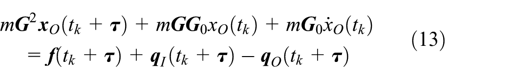
The dynamics equation of a lumped mass m undergoing a one-dimensional motion in x-direction shown in Figure 1(a) can be written as

m {\overset{\cdot\cdot}{x}}_{O} = f + q_{I} - q_{O}

(12)

where f is the applied force, and $q_{I}$ and $q_{O}$ are forces acting at the body input I and output O. By applying equation (11), we get

\begin{matrix} m G^{2} x_{O} (t_{k} + τ) + m G G_{0} x_{O} (t_{k}) + m G_{0} {\overset{\cdot}{x}}_{O} (t_{k}) \\ = f (t_{k} + τ) + q_{I} (t_{k} + τ) - q_{O} (t_{k} + τ) \end{matrix}

(13)

Figure 1.

Models of four basic elements: (a) lumped mass, (b) spring–damper, (c) truss element, and (d) beam element.

For the lumped mass, the displacement of the output point equals that of the input point, that is

x_{O} (t_{k} + τ) = x_{I} (t_{k} + τ)

(14)

Thus, equation (13) may be rewritten as

\begin{matrix} q_{O} (t_{k} + τ) = - m G^{2} x_{I} (t_{k} + τ) + q_{I} (t_{k} + τ) + f (t_{k} + τ) \\ - m G G_{0} x_{O} (t_{k}) - m G_{0} {\overset{\cdot}{x}}_{O} (t_{k}) \end{matrix}

(15)

By defining the state vector as

z = {[x^{T} (t_{k} + τ), q^{T} (t_{k} + τ), 1]}^{T}

(16)

equations (14) and (15) may be summarized as transfer equation

z_{O} = U z_{I}

(17)

where the transfer matrix of the lumped mass undergoing one-dimensional motion based on DQ-DT-TMM is

U = [\begin{matrix} \underset{(N - 1) \times (N - 1)}{I} & \underset{(N - 1) \times (N - 1)}{O} & \underset{(N - 1)}{O} \\ \underset{(N - 1) \times (N - 1)}{- m G^{2}} & \underset{(N - 1) \times (N - 1)}{I} & \underset{(N - 1)}{f (t_{k} + τ) - m G G_{0} x_{O} (t_{k}) - m G_{0} {\overset{\cdot}{x}}_{O} (t_{k})} \\ {\underset{(N - 1)}{O}}^{T} & {\underset{(N - 1)}{O}}^{T} & 1 \end{matrix}]

(18)

It should be noted that equation (17) provides a linear relationship between the state vectors of input and output points for the time sequence $t_{k} + τ_{2}, t_{k} + τ_{3}, \dots, t_{k} + τ_{N}$ , since all components of the $[2 (N - 1) + 1] \times [2 (N - 1) + 1]$ transfer matrix (18) are known at time instant $t_{k}$ .

Linear spring–damper in one-dimensional motion

The equilibrium equation of a linear spring–damper in one-dimensional direction (Figure 1(b)) can be written as

k' (x_{O} - x_{I}) + c ({\overset{\cdot}{x}}_{O} - {\overset{\cdot}{x}}_{I}) = - q_{I}

(19)

and

q_{I} = q_{O}

(20)

where $k'$ denotes the stiffness coefficient of the linear spring, $c$ the damping coefficient of the linear damper, $x$ and $\overset{\cdot}{x}$ are displacement and velocity of output point O and input point I, and $q_{I}$ and $q_{O}$ are forces acting on the spring–damper component.

By using equation (8), equation (19) becomes

\begin{matrix} k' [x_{O} (t_{k} + τ) - x_{I} (t_{k} + τ)] + c [G x_{O} (t_{k} + τ) \\ + G_{0} x_{O} (t_{k}) - G x_{I} (t_{k} + τ) \\ - G_{0} x_{I} (t_{k})] = - q_{I} (t_{k} + τ) \end{matrix}

(21)

\begin{matrix} (k' I + c G) x_{O} (t_{k} + τ) = - q_{I} (t_{k} + τ) + (k' I + c G) x_{I} \\ (t_{k} + τ) + c G_{0} [x_{I} (t_{k}) - x_{O} (t_{k})] \end{matrix}

(22)

With definition (equation (16)), equations (20) and (22) may also be summarized as transfer equation (17), where the transfer matrix of the linear spring–damper is

U = [\begin{matrix} \underset{(N - 1) \times (N - 1)}{I} & - {(\underset{(N - 1) \times (N - 1)}{k' I} + c G)}^{- 1} & c {(\underset{(N - 1) \times (N - 1)}{k' I} + c G)}^{- 1} G_{0} (x_{I} (t_{k}) - x_{O} (t_{k})) \\ \underset{(N - 1) \times (N - 1)}{O} & \underset{(N - 1) \times (N - 1)}{I} & \underset{(N - 1)}{O} \\ {\underset{(N - 1)}{O}}^{T} & {\underset{(N - 1)}{O}}^{T} & 1 \end{matrix}]

(23)

One-dimensional truss element

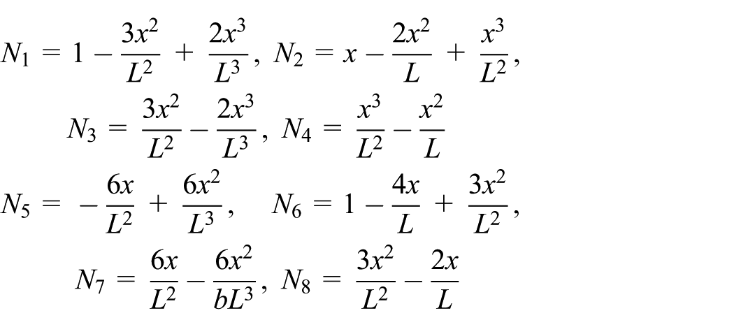
Next, the one-dimensional rod in Figure 1(c) with the cross-section area A and length L = 2a is considered. The axial displacements may be interpolated by Lagrange shape functions as⁵³

u (x) = N (x) u^{e}

(24)

where the nodal displacement vector is defined as

u^{e} = {[u_{I}, u_{O}]}^{T}

(25)

and the shape functions are

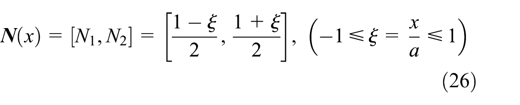
N (x) = [N_{1}, N_{2}] = [\frac{1 - ξ}{2}, \frac{1 + ξ}{2}], (- 1 \leq ξ = \frac{x}{a} \leq 1)

(26)

Using the energy rule and equation (24), the stiffness matrix $K^{e}$ and the mass matrix $M^{e}$ of the one-dimensional rod can be deduced as

\begin{matrix} K^{e} = \frac{EA}{L} [\begin{matrix} 1 & - 1 \\ - 1 & 1 \end{matrix}] = [\begin{matrix} k_{11}^{e} & k_{12}^{e} \\ k_{21}^{e} & k_{22}^{e} \end{matrix}], \\ M^{e} = \frac{ρ AL}{2} [\begin{matrix} \frac{2}{3} & \frac{1}{3} \\ \frac{1}{3} & \frac{2}{3} \end{matrix}] = [\begin{matrix} m_{11}^{e} & m_{12}^{e} \\ m_{21}^{e} & m_{22}^{e} \end{matrix}] \end{matrix}

(27)

where $E$ and $ρ$ are elastic modulus and density. According to the virtual work principle, the external force $f^{e} = [f_{I}, f_{O}]^{T}$ and the internal force $q^{e} = [q_{I}, q_{O}]^{T}$ lead to the dynamics equation

M^{e} {\overset{\cdot\cdot}{u}}^{e} + C^{e} {\overset{\cdot}{u}}^{e} + K^{e} u^{e} = f^{e} + q^{e}

(28)

where $C^{e}$ is a damping matrix. Application to the grid points yields

\begin{matrix} M^{e} [\begin{matrix} {\overset{\cdot\cdot}{u}}_{I} (t_{k} + τ_{j}) \\ {\overset{\cdot\cdot}{u}}_{O} (t_{k} + τ_{j}) \end{matrix}] + C^{e} [\begin{matrix} {\overset{\cdot}{u}}_{I} (t_{k} + τ_{j}) \\ {\overset{\cdot}{u}}_{O} (t_{k} + τ_{j}) \end{matrix}] + K^{e} [\begin{matrix} u_{I} (t_{k} + τ_{j}) \\ u_{O} (t_{k} + τ_{j}) \end{matrix}] \\ = [\begin{matrix} f_{I} (t_{k} + τ_{j}) \\ f_{O} (t_{k} + τ_{j}) \end{matrix}] + [\begin{matrix} q_{I} (t_{k} + τ_{j}) \\ q_{O} (t_{k} + τ_{j}) \end{matrix}] \end{matrix}

(29)

Using equations (8) and (11), this can be rewritten and summarized as

\bar{H} {\bar{u}}^{e} (t_{k} + τ) + \bar{H'} = \bar{f} (t_{k} + τ) + \bar{q} (t_{k} + τ)

(30)

where

\begin{matrix} \bar{H} = {\bar{M}}^{e} {\bar{G}}^{2} + {\bar{C}}^{e} \bar{G} + {\bar{K}}^{e}, \bar{H'} = ({\bar{M}}^{e} \bar{G} {\bar{G}}_{0} + {\bar{C}}^{e} {\bar{G}}_{0}) {\bar{u}}^{e} (t_{k}) \\ + {\bar{M}}^{e} {\bar{G}}_{0} {\overset{\cdot}{\bar{u}}}^{e} (t_{k}) \\ {\bar{M}}^{e} = [\begin{matrix} M^{e} & O & \dots & O \\ O & M^{e} & \dots & O \\ ⋮ & ⋮ & ⋱ & ⋮ \\ O & O & \dots & M^{e} \end{matrix}], {\bar{C}}^{e} = [\begin{matrix} C^{e} & O & \dots & O \\ O & C^{e} & \dots & O \\ ⋮ & ⋮ & ⋱ & ⋮ \\ O & O & \dots & C^{e} \end{matrix}], \\ {\bar{K}}^{e} = [\begin{matrix} K^{e} & O & \dots & O \\ O & K^{e} & \dots & O \\ ⋮ & ⋮ & ⋱ & ⋮ \\ O & O & \dots & K^{e} \end{matrix}] \\ \bar{G} = [\begin{matrix} G_{22}^{(1)} I & G_{23}^{(1)} I & \dots & G_{2 N}^{(1)} I \\ G_{32}^{(1)} I & G_{33}^{(1)} I & \dots & G_{3 N}^{(1)} I \\ ⋮ & ⋮ & ⋱ & ⋮ \\ G_{N 2}^{(1)} I & G_{N 3}^{(1)} I & \dots & G_{NN}^{(1)} I \end{matrix}], {\bar{G}}_{0} = [\begin{matrix} G_{21}^{(1)} I \\ G_{31}^{(1)} I \\ ⋮ \\ G_{N 1}^{(1)} I \end{matrix}] \\ {\bar{u}}^{e} (t_{k} + τ) = [\begin{matrix} u_{I} (t_{k} + τ_{2}) \\ u_{O} (t_{k} + τ_{2}) \\ ⋮ \\ u_{I} (t_{k} + τ_{N}) \\ u_{O} (t_{k} + τ_{N}) \end{matrix}], \bar{f} (t_{k} + τ) \\ = [\begin{matrix} f_{I} (t_{k} + τ_{2}) \\ f_{O} (t_{k} + τ_{2}) \\ ⋮ \\ f_{I} (t_{k} + τ_{N}) \\ f_{O} (t_{k} + τ_{N}) \end{matrix}], \bar{q} (t_{k} + τ) = = [\begin{matrix} q_{I} (t_{k} + τ_{2}) \\ q_{O} (t_{k} + τ_{2}) \\ ⋮ \\ q_{I} (t_{k} + τ_{N}) \\ q_{O} (t_{k} + τ_{N}) \end{matrix}] \end{matrix}

(31)

By reordering these vectors as

\begin{matrix} u^{e} (t_{k} + τ) = [\begin{matrix} u_{I}^{e} (t_{k} + τ) \\ u_{O}^{e} (t_{k} + τ) \end{matrix}], f^{e} (t_{k} + τ) = [\begin{matrix} f_{I}^{e} (t_{k} + τ) \\ f_{O}^{e} (t_{k} + τ) \end{matrix}], \\ q^{e} (t_{k} + τ) = [\begin{matrix} q_{I}^{e} (t_{k} + τ) \\ q_{O}^{e} (t_{k} + τ) \end{matrix}] \end{matrix}

(32)

equation (30) can be rewritten as

\begin{matrix} [\begin{matrix} H_{11} & H_{12} \\ H_{21} & H_{22} \end{matrix}] [\begin{matrix} u_{I}^{e} (t_{k} + τ) \\ u_{O}^{e} (t_{k} + τ) \end{matrix}] + [\begin{matrix} {H'}_{1} \\ {H'}_{2} \end{matrix}] = [\begin{matrix} f_{I}^{e} (t_{k} + τ) \\ {f_{O}}^{e} (t_{k} + τ) \end{matrix}] \\ + [\begin{matrix} q_{I}^{e} (t_{k} + τ) \\ q_{O}^{e} (t_{k} + τ) \end{matrix}] \end{matrix}

(33)

The 2(N – 1) + 1 state vector of the one-dimensional two-node rod at input I and output O points can be defined analogously to equation (16) as

z_{i} = {[u_{i}^{eT} (t_{k} + τ), q_{i}^{eT} (t_{k} + τ), 1]}^{T}, i = I, O

(34)

From equation (33) we may deduce

\begin{matrix} H_{12} u_{O}^{e} (t_{k} + τ) = - H_{11} u_{I}^{e} (t_{k} + τ) + q_{I}^{e} (t_{k} + τ) \\ + f_{I}^{e} (t_{k} + τ) - {H'}_{1} \end{matrix}

(35)

to be solved for $u_{O}^{e} (t_{k} + τ)$ and substituted in the second equation, reordered as

\begin{matrix} q_{O}^{e} (t_{k} + τ) = (H_{21} - H_{22} H_{12}^{- 1} H_{11}) u_{I}^{e} (t_{k} + τ) \\ + H_{22} H_{12}^{- 1} q_{I}^{e} (t_{k} + τ) \\ + H_{22} H_{12}^{- 1} [f_{I}^{e} (t_{k} + τ) - H'] + {H'}_{2} - {f_{O}}^{e} (t_{k} + τ) \end{matrix}

(36)

By using the condition of displacement continuum and the law of action and reaction at a point, equations (35) and (36) may be summarized as equation (17) with transfer matrix

U = [\begin{matrix} - H_{12}^{- 1} H_{11} & H_{12}^{- 1} & H_{12}^{- 1} [f_{I}^{e} (t_{k} + τ) - {H'}_{1}] \\ H_{22} H_{12}^{- 1} H_{11} - H_{21} & - H_{22} H_{12}^{- 1} & f_{O}^{e} (t_{k} + τ) - H_{22} H_{12}^{- 1} (f_{I}^{e} (t_{k} + τ) - H') - {H'}_{2} \\ O & O & 1 \end{matrix}]

(37)

Beam element

In order to extend the method to simulation of beam vibrations, the Euler–Bernoulli beam neglecting shear deformation and rotary inertia effects may be introduced in Figure 1(d). The displacements in z-direction and slopes $θ (x) = \partial w / \partial w \partial x \partial x$ can be expressed approximately as⁵³

{[w_{0}, θ_{0}]}^{T} = [\begin{matrix} N_{1} & N_{2} & N_{3} & N_{4} \\ N_{5} & N_{6} & N_{7} & N_{8} \end{matrix}] u^{e}

(38)

based on the nodal displacement vector

u^{e} = {[w_{I}, θ_{I}, w_{O}, θ_{O}]}^{T}

(39)

and the shape functions

\begin{matrix} N_{1} = 1 - \frac{3 x^{2}}{L^{2}} + \frac{2 x^{3}}{L^{3}}, N_{2} = x - \frac{2 x^{2}}{L} + \frac{x^{3}}{L^{2}}, \\ N_{3} = \frac{3 x^{2}}{L^{2}} - \frac{2 x^{3}}{L^{3}}, N_{4} = \frac{x^{3}}{L^{2}} - \frac{x^{2}}{L} \\ N_{5} = - \frac{6 x}{L^{2}} + \frac{6 x^{2}}{L^{3}}, N_{6} = 1 - \frac{4 x}{L} + \frac{3 x^{2}}{L^{2}}, \\ N_{7} = \frac{6 x}{L^{2}} - \frac{6 x^{2}}{b L^{3}}, N_{8} = \frac{3 x^{2}}{L^{2}} - \frac{2 x}{L} \end{matrix}

Application of mechanics law results in dynamics equation (28) with stiffness and mass matrices

\begin{matrix} K^{e} = \frac{E I_{z}}{L^{3}} [\begin{matrix} 12 & 6 L & - 12 & 6 L \\ 6 L & 4 L^{2} & - 6 L & 2 L^{2} \\ - 12 & - 6 L & 12 & - 6 L \\ 6 L & 2 L^{2} & - 6 L & 4 L^{2} \end{matrix}], \\ M^{e} = \frac{ρ AL}{420} [\begin{matrix} 156 & 22 L & 54 & - 13 L \\ 22 L & 4 L^{2} & 13 L & - 3 L^{2} \\ 54 & 13 L & 156 & - 22 L \\ - 13 L & - 3 L^{2} & - 22 L & 4 L^{2} \end{matrix}] \end{matrix}

(40)

of the two-node beam element, where $E$ and $ρ$ are elastic modulus and density, $I_{z}$ , $A$ , and $L$ denote moment of inertia, area of the beam section, and length. The equivalent internal forces in nodes I and O are

q^{e} = {[f_{I}, M_{I}, f_{O}, M_{O}]}^{T}

(41)

which can be seen in Figure 1(d). The deduction of the corresponding transfer equation is similar to section “One-dimensional truss element.”

Algorithm for vibration analysis

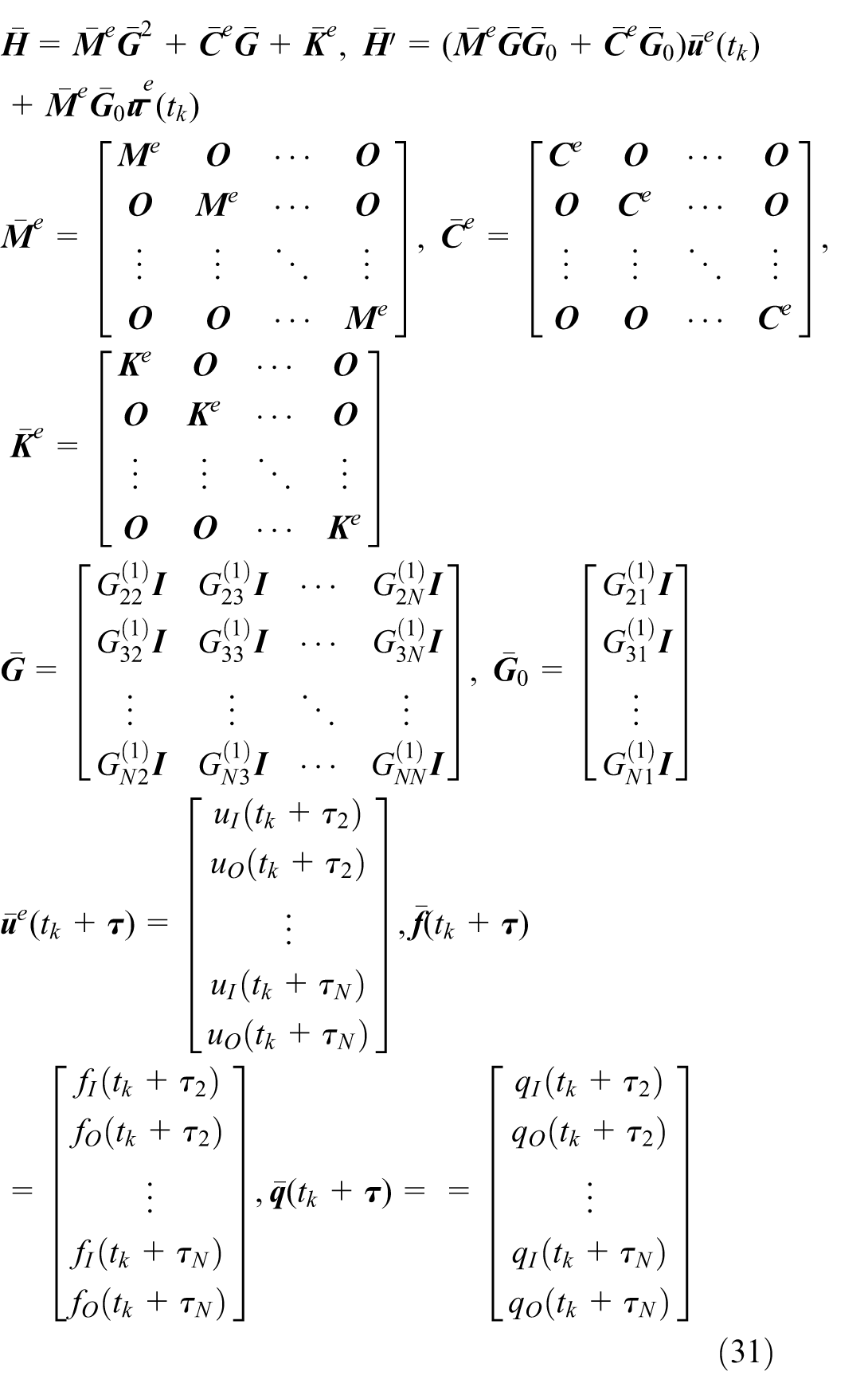
The global transfer equation of a chain system consisting of the $N_{e}$ elements, where each element is described by a transfer relation (equation (18)), can be obtained by recursively substituting intermediate states. Let $z_{I}$ , $z_{O}$ be the boundary states, then from the identities $z_{O, i - 1} = z_{I, i}$ and $z_{O} = z_{N_{e}}, z_{I} = z_{1}$ we get

z_{O} \equiv z_{O, N_{e}} = U_{N_{e}} z_{I, N_{e}} \equiv U_{N_{e}} z_{O, N_{e} - 1} = \dots = : U_{all} z_{I}

(42)

where the global transfer matrix of the system can be expressed as production of element transfer matrices $U_{i}$

U_{all} = Π_{i = 1}^{N_{e}} U_{i}

(43)

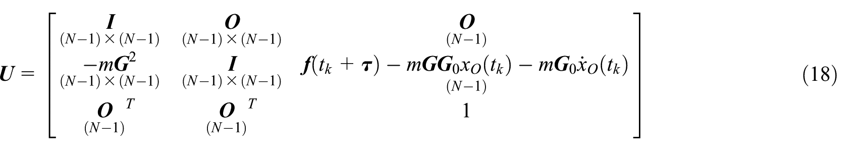
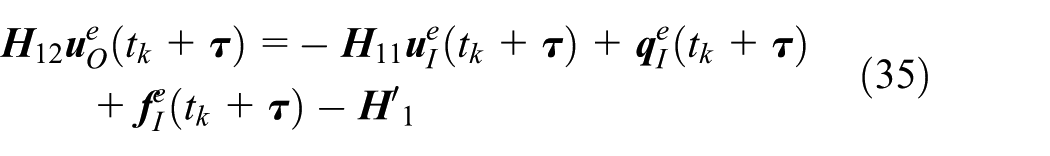
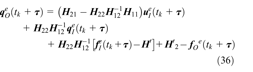
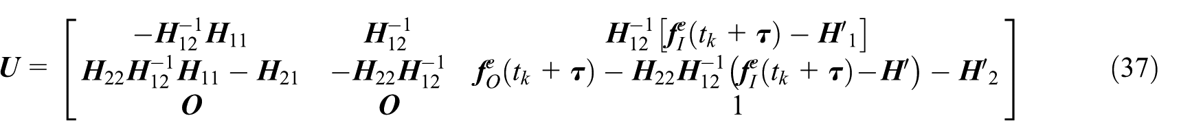
Generally, half of the components in the boundary state vectors are known. By resolving the algebraic equation (42), the other half of the boundary states can be obtained. However, with increase in the number $N_{e}$ of elements, rounding errors may increase by the multiplication of transfer matrices $U_{i}$ in equation (43). These errors may enlarge the accumulated error to such an extent that computation results become invalid. Riccati transformation is an important tool to improve the performance of numerical stability in transfer computations.^3,18

Riccati DQ-DT-TMM

To introduce the Riccati transformation into equation (17), the state vector can be divided into three parts

z = [z^{T}, z^{T}, 1]^{T}

(44)

where $z^{1}$ includes the known state variables, for example, known boundary states, and $z^{2}$ the unknown state variables. Then, any element transfer equation may be reordered as

[\begin{matrix} z_{i}^{1} \\ z_{i}^{2} \end{matrix}] = [\begin{matrix} {\bar{U}}_{11}^{i} & {\bar{U}}_{12}^{i} \\ {\bar{U}}_{21}^{i} & {\bar{U}}_{22}^{i} \end{matrix}] [\begin{matrix} z_{i - 1}^{1} \\ z_{i - 1}^{2} \end{matrix}] + [\begin{matrix} {\bar{U}}_{1}^{i} \\ {\bar{U}}_{2}^{i} \end{matrix}]

(45)

where ${\bar{U}}_{1}^{i}, {\bar{U}}_{2}^{i}$ correspond to the last column of transfer matrices (18), (23), or (37). Assume that known states may be expressed by unknown states as

z_{i - 1}^{1} = S_{i - 1} z_{i - 1}^{2} + P_{i - 1}

(46)

Substitution into equation (46) yields

z_{i}^{2} = ({\bar{U}}_{21}^{i} S_{i - 1} + {\bar{U}}_{22}^{i}) z_{i - 1}^{2} + {\bar{U}}_{21}^{i} P_{i - 1} + {\bar{U}}_{2}^{i}

(47)

or after rearrangement

\begin{matrix} z_{i - 1}^{2} = {({\bar{U}}_{21}^{i} S_{i - 1} + {\bar{U}}_{22}^{i})}^{- 1} z_{i}^{2} - {({\bar{U}}_{21}^{i} S_{i - 1} + {\bar{U}}_{22}^{i})}^{- 1} \\ ({\bar{U}}_{21}^{i} P_{i - 1} + {\bar{U}}_{i}^{2}) \end{matrix}

(48)

With abbreviations

T_{i} = {({\bar{U}}_{21}^{i} S_{i - 1} + {\bar{U}}_{22}^{i})}^{- 1}, Q_{i} = - ({\bar{U}}_{21}^{i} P_{i - 1} + {\bar{U}}_{i}^{2})

(49)

this may be simplified to

z_{i - 1}^{2} = T_{i} (z_{i}^{2} + Q_{i})

(50)

By substituting equations (46), (47), and (50) into equation (45), we can obtain

\begin{matrix} z_{i}^{1} = ({\bar{U}}_{11}^{i} S_{i - 1} + {\bar{U}}_{12}^{i}) T_{i} z_{i}^{2} + {\bar{U}}_{11}^{i} P_{i - 1} + {\bar{U}}_{i}^{1} \\ + ({\bar{U}}_{11}^{i} S_{i - 1} + {\bar{U}}_{12}^{i}) T_{i} Q_{i} \end{matrix}

(51)

By comparing equation (47) with (51), recursive transfer equations can be deduced for

S_{i} = ({\bar{U}}_{11}^{i} S_{i - 1} + {\bar{U}}_{12}^{i}) T_{i}

(52)

P_{i} = {\bar{U}}_{11}^{i} P_{i - 1} + {\bar{U}}_{i}^{1} + S_{i} Q_{i}

(53)

Equations (47), (49), (52), and (53) are the formulas of the Riccati transform matrix method.

Algorithmic analysis

In order to use equations (52) and (53) recursively, matrices P and S of the system boundary must be given first. According to equation (44), $z_{0}^{1}$ in system boundaries is always known, where subscript 0 denotes a boundary end of the system. According to equation (46), the matrices P and S of this system boundary end can then be defined as

P_{0} = z_{0}^{1}, S_{0} = O

(54)

where $O$ is the zero matrix.

By using equations (52) and (53) repeatedly, the matrices $S_{i}, P_{i}$ at any node $i$ can be obtained. Especially matrices $S_{N_{e}}, P_{N_{e}}$ at the last node $N_{e}$ , being also a system boundary, can be substituted into equation (46) as

z_{N_{e}}^{1} = S_{N_{e}} z_{N_{e}}^{2} + P_{N_{e}}

(55)

This is an algebraic equation reflecting the relationship between the state variables at system boundary, where half of the state variables summarized in $z_{N_{e}}^{1}$ is known generally. Thus, the unknown elements $z_{N_{e}}^{2}$ can be obtained by solving equation (55). By using $T_{i}$ and $Q_{i}$ , $z_{i - 1}^{2}$ at any internal node $i = N_{e}, N_{e} -$ $1, \dots, 2, 1$ can be obtained by equation (50), and the corresponding $z_{i - 1}^{1}$ can be obtained from equation (46).

Algorithm process

According to the formulas given above, the motion quantities of a vibration system at different instants can be obtained as follows.

Decide the properties of the vibration system and the parameters of the computational method, such as the number $N$ and location of grid points determining $G_{0}$ and $G$ .

Set k = 1 and the initial conditions $u (t_{1})$ , $\overset{\cdot}{u} (t_{1})$ .

According to the system boundary condition determining equation (54) and the element transfer matrices, the Riccati transform matrices $S_{i}$ , $P_{i}$ , $T_{i}$ , and $Q_{i}$ at any connecting node $i$ can be obtained by equations (49), (52), and (53), respectively.

Solve equation (55) and obtain the unknown elements of last nodal state vector.

Compute state variable of all nodes at time $t_{k} + τ$ by using equations (47) and (52).

According to equations (8) and (11), compute the values of $\overset{\cdot}{u} (t_{k} + τ)$ by applying equation (8) to the displacements $u (t_{k} + τ)$ .

Let $k : = k + 1$ , set the computed values $u (t_{k} + τ_{N})$ , $\overset{\cdot}{u} (t_{k} + τ_{N})$ as new initial conditions for the next time interval and return to step 3, until the time required for complete analysis is arrived.

Numerical examples

Vibration of a spring–damper–mass system

Single-DOF system

In order to verify the method, first we compute the free vibration of a linear spring–damper–mass system with 1 DOF. The properties of the system are $m = 1 kg$ , $k' = 1 \times 10^{4} N / m$ , and $c = 1 N / m / s$ , and the initial conditions are assumed to be $x (0) = 0.1 m$ and $\overset{\cdot}{x} (0) = 1 m / s$ . The total energy can be expressed as

E_{0} = \frac{1}{2} m {\overset{\cdot}{x}}^{2} + \frac{1}{2} k' x^{2}

(56)

Figures 2 and 3 show the displacement and the total energy at different time points for $Δ T = T / 80$ , $T = 0.7 s$ where Newmark method $(γ = 0.5, β = 0.25)$ , fourth-order explicit Runge–Kutta method (RK4), and DQ-DT-TMM are compared to the exact result. Stars are the result of DQ-DT-TMM with $N = 4$ Gauss grid points (scheme 4 in section “DQ”). It can be found in Figure 3 that the total energy is exhausted continuously by the effect of the damper and takes on the slight wave pattern, which is induced by the periodic velocity and damped force. Obviously, the Newmark method increases the motion period and total energy, whereas the Runge–Kutta method weakens the vibration amplitude and total energy. The data of DQ-DT-TMM agree best with the exact solution among these three numerical methods.

Figure 2.

Displacement curve by four different methods.

Figure 3.

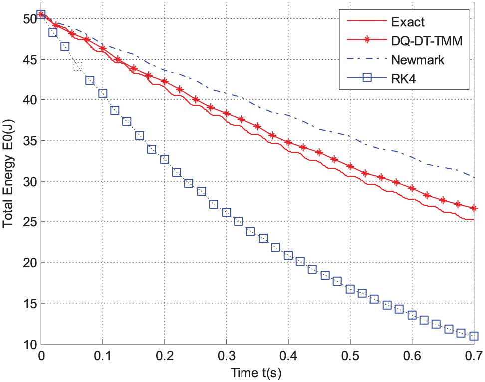
Total energy curve by four different methods.

Table 1 lists the absolute percentage errors of the systems total energy at end time $T = 0.7 s$ for different time step sizes $Δ T$ . When the time step size decreases, DQ-DT-TMM shows the best convergence characteristic and has highest computational precision for all time steps.

Table 1.

Absolute percentage errors in total energy of 1-DOF system at end time.

$Δ T$	$\frac{T}{80}$	$\frac{T}{100}$	$\frac{T}{150}$	$\frac{T}{200}$	$\frac{T}{500}$	$\frac{T}{1000}$	$\frac{T}{5000}$	$\frac{T}{10, 000}$
DQ-DT-TMM	20.035	7.371	1.065	0.263	0.003	0.000	0.000	0.000
Newmark	33.399	22.787	10.528	7.015	1.005	0.232	0.009	0.002
Runge–Kutta	96.806	69.817	15.339	3.908	0.038	0.001	0.000	0.000

DOF: degree of freedom; DQ-DT-TMM: differential quadrature discrete time transfer matrix method.

In Table 2, different numbers N of grid points and grid point schemes from section “DQ” in DQ-DT-TMM and HDQ-DT-TMM are analyzed. Both DQM and HDQM in DT-TMM have similar computational features. The Gauss grid point scheme 4 has the best convergence performance along the increasing number of grid points $N$ . The Chebyshev–Gauss–Lobatto grid point 2 scheme has the highest error precision for $N = 4$ . In order to simulate with high efficiency, HDQM with the grid point scheme 4 and $N = 5$ may be recommended and will be used in the remainder of the article.

Table 2.

Absolute percentage errors in total energy of 1-DOF system at end time with $Δ T = T / T 50 50$ .

Method	Grid scheme	N
		4	5	6	7	8	9	10
DQ-DT-TMM	1	*	*	5.428	1.235	0.058	0.010	0.000
	2	28.859	25.1797	0.565	0.129	0.003	0.000	0.000
	3	*	92.915	2.666	0.534	0.017	0.002	0.000
	4	86.255	4.803	0.069	0.001	0.000	0.000	0.000
	5	95.460	52.665	1.326	0.284	0.008	0.001	0.000
HDQ-DT-TMM	1	*	*	5.426	1.234	0.058	0.010	0.000
	2	28.856	25.171	0.565	0.129	0.003	0.000	0.000
	3	*	92.875	2.665	0.534	0.017	0.002	0.000
	4	86.252	4.802	0.069	0.001	0.000	0.000	0.000
	5	95.441	52.645	1.325	0.284	0.008	0.001	0.000

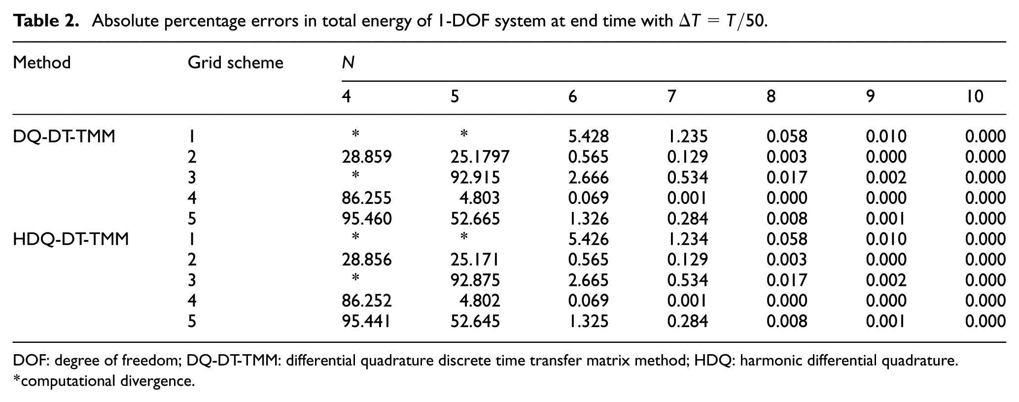
DOF: degree of freedom; DQ-DT-TMM: differential quadrature discrete time transfer matrix method; HDQ: harmonic differential quadrature.

computational divergence.

Multi-DOF system

The 3-DOF spring-mass system in Figure 4 may be regarded as an example of a multi-DOF system. Its structural parameters are $m_{1} = m_{2} = m_{3} = 10 kg$ , $k_{1} = k_{2} = k_{3} = 4 \times 10^{3} N / m$ , and the initial conditions are $x_{1} (0) = 1 m$ , $x_{2} (0) = x_{3} (0) = 0 m$ , and ${\overset{\cdot}{x}}_{1} (0) = {\overset{\cdot}{x}}_{2} (0) = {\overset{\cdot}{x}}_{3} (0) = 0 m / s$ . If no applied forces are considered in the system, the exact analytical solutions will be found in classical text books.⁵⁴

Figure 4.

Three-degree-of-freedom spring–mass system.

From Figure 5, we can clearly find that the Newmark method and DQ-DT-TMM have worst and best computational precision among the three numerical methods, respectively. Table 3 showing errors of the mechanically constant total energy demonstrates that DQ-DT-TMM has a better conservative characteristic than the Runge–Kutta method when a large time step size is used.

Figure 5.

System displacement curves for the 3-DOF system.

Table 3.

Absolute percentage errors in total energy of 3-DOF system at end time T = 5 s.

$Δ T$	$\frac{T}{100}$	$\frac{T}{150}$	$\frac{T}{200}$	$\frac{T}{250}$	$\frac{T}{300}$	$\frac{T}{400}$	$\frac{T}{600}$	$\frac{T}{800}$
DQ-DT-TMM	2.441	0.157	0.022	0.005	0.001	0.000	0.000	0.000
Runge–Kutta	98.372	76.130	47.926	22.886	10.545	2.721	0.370	0.088

DOF: degree of freedom; DQ-DT-TMM: differential quadrature discrete time transfer matrix method.

Vibration of one-dimensional rod

An aluminum rod with Young’s modulus $E = 71.08 GPa$ , diameter $d = 20 mm$ , length $l = 1 m$ , and density $ρ = 2710 kg / m^{3}$ is struck by a steel ball with radius $R = 1.5 cm$ and mass $m = 0.11 kg$ . The rod can be regarded as a free body excited by an impact force as shown in Figure 6(a), which has been analyzed by experiment and a theoretical method.⁵⁵

Figure 6.

Vibration models of two structure components: (a) impact on one-dimensional rod and (b) vibration of a slender beam.

Figure 7 shows the time history of displacement and velocity at the right end of the rod obtained by the fourth order explicit Runge–Kutta method, Newmark $(γ = 0.5, β = 0.25)$ , and DQ-DT-TMM with $Δ T = T / 200$ as well as the experiment⁵⁵ and $N_{e} = 200$ elements. The red solid line denoting experimental data may be regarded as reference data. All three simulation methods show the phenomenon of wave propagation after impact, and DQ-DT-TMM solves the response most precisely.

Figure 7.

Displacement (a) and velocity (b) curves of rod simulated by three methods and experiment.

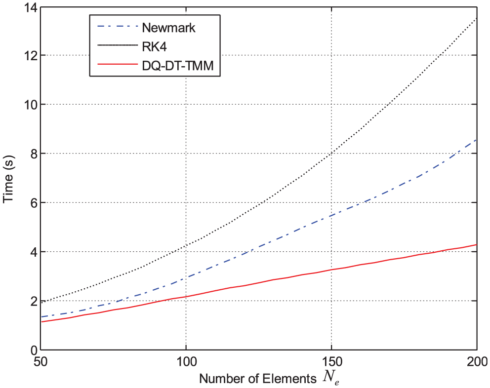
Figure 8 presents a comparison of the CPU time for the three methods when the number $N_{e}$ of the truss elements changes from 50 to 200. Obviously, the computational speed of DQ-DT-TMM is faster than that of the other two methods for all numbers of truss elements. Moreover, the CPU time of DQ-DT-TMM increases only linearly with the number of truss elements, whereas CPU time of Runge–Kutta and Newmark methods will increase more rapidly.

Figure 8.

Comparison of the CPU time for impacted rod.

Vibration of bending beam

As shown in Figure 6(b), a vertical force is applied at the midpoint of the horizontal beam with two simply supported ends.

f (t) = {\begin{matrix} 1000 \sin (\frac{π}{t_{1}} t) + 5000 \sin (\frac{π}{t_{2}} t) for t \leq t_{1}, t_{1} = 0.14 s, t_{2} = 0.005 s \\ 0 for t_{1} < t \leq 0.4 s, t_{1} = 0.14 s \end{matrix}

(57)

The beam is homogeneous, and its cross section is circular with diameter 30 mm. The length, density, and Young’s modulus of the beam are 3 m, 7810 kg/m³, and 71.08 GPa, respectively, where $N_{e} = 4$ elements are used.

The bending response of the beam can be obtained analytically⁵⁴ as well as by DQ-DT-TMM, Newmark $(γ = 0.5, β = 0.25)$ , and fourth order Runge–Kutta methods for $Δ T = T / 600$ and $T = 0.4 s$ . Figure 9 shows the transverse displacement $w$ and velocity $\overset{\cdot}{w}$ of the midpoint of the beam. Again the data of DQ-DT-TMM agree better with the exact results than that of the other simulations.

Figure 9.

Displacement (a) and velocity (b) curves of the beam midpoint.

When the number $N_{e}$ of beam elements is more than 4, the Runge–Kutta method cannot give any convergent result for the time step size $Δ T = T / 600$ . The CPU time for different beam element numbers $N_{e}$ from 100 to 220 by Newmark and DQ-DT-TMM are displayed in Figure 10. It can be noted that the CPU time of DQ-DT-TMM is less than that of Newmark when the number of beam elements is much more than 144. Furthermore, the CPU time of Newmark increases faster than that of DQ-DT-TMM.

Figure 10.

Comparison of the CPU time for the beam vibration.

Conclusion

By the combination of the DQ time integration method and the DT-TMM, a new method called DQ-DT-TMM is developed. Application to single- and multi-DOF systems as well as impacted rod and beam illustrates that DQ-DT-TMM is an efficient technology for simulating transient vibration responses. In order to state the basic idea of the method conveniently, the article is limited to linear vibrations. The nonlinear vibration for complex structures will be resolved in a forthcoming article. The highlights of DQ-DT-TMM are efficient computation, good numerical stability, and high calculation precision compared to Runge–Kutta and Newmark methods.

Footnotes

Handling Editor: Chuanzeng Zhang

Declaration of conflicting interests

The author(s) declared no potential conflicts of interest with respect to the research, authorship, and/or publication of this article.

Funding

The author(s) disclosed receipt of the following financial support for the research, authorship, and/or publication of this article: The research was financed by Science Challenge Project in China (TZ2016006-0104), Natural Science Foundation of China (11472135), and Natural Science Foundation of Jiangsu Province, China (BK20130911).

ORCID iDs

Xue Rui

Guoping Wang

Bin He

References

Pestel

Leckie

. Matrix methods in elastomechanics. New York: McGraw-Hill, 1963.

Uhrig

. The transfer matrix method seen as one method of structural analysis among others. J Sound Vib 1966; 4: 136–148.

Horner

Pilkey

. The Riccati transfer matrix method. J Mech Design 1978; 100: 297–302.

Dokainish

. A new approach for plate vibrations: combination of transfer matrix and finite-element technique. J Eng Ind 1972; 94: 526–530.

McDaniel

Eversole

. A combined finite element-transfer matrix structural analysis method. J Sound Vib 1977; 51: 157–169.

Ohga

Shigematsu

Hara

. Structural analysis by a combined finite element-transfer matrix method. Comput Struct 1983; 17: 321–326.

Kumar

Sankar

. A new transfer matrix method for response analysis of large dynamic systems. Comput Struct 1986; 23: 545–552.

Fang

. Dynamic analysis of structures with uncertain parameters using the transfer matrix method. Comput Struct 1995; 55: 1037–1044.

Rong

Rui

Wang

et al . Discrete time transfer matrix method for dynamics of multibody system with real-time control. J Sound Vib 2010; 329: 627–643.

10.

Yildirim

Sancaktar

Kiral

. Free vibration analysis of symmetric cross-ply laminated composite beams with the help of the transfer matrix approach. Int J Numer Meth Biomed Eng 1999; 15: 651–660.

11.

Rui

Wang

et al . Transfer matrix method for linear multibody system. Multibody Syst Dyn 2008; 19: 179–207.

12.

Tsai

Tsau

Chen

. Vibration analysis of a beam with partially distributed internal viscous damping. Int J Mech Sci 2009; 51: 907–914.

13.

Liu

et al . Vibration analysis of pipelines with arbitrary branches by absorbing transfer matrix method. J Sound Vib 2013; 332: 6519–6536.

14.

Thinh

Nguyen

. Dynamic stiffness matrix of continuous element for vibration of thick cross-ply laminated composite cylindrical shells. Compos Struct 2013; 98: 93–102.

15.

Wang

Kang

Sun

et al . Modeling and parameter analysis of in-plane dynamics of a suspension bridge with transfer matrix method. Acta Mech 2014; 225: 3423–3435.

16.

Zhi

Meng

et al . Transient response analysis of large-scale rotor-bearing system with strong non-linear elements by a transfer matrix-Newmark formulation itegration method. J Sound Vib 2003; 259: 559–570.

17.

Rui

et al . Discrete time transfer matrix method for multibody system dynamics. Multibody Syst Dyn 2005; 14: 317–344.

18.

Rui

Wang

. Riccati discrete time transfer matrix method for elastic beam undergoing large overall motion. Multibody Syst Dyn 2007; 18: 579–598.

19.

Huang

Jiang

. Analysis of source models for two-dimensional acoustic systems using the transfer matrix method. J Sound Vib 2007; 306: 215–226.

20.

Yong

Qibai

Minggang

et al . Transfer matrix approach of vibration isolation analysis of periodic composite structure. Arch Appl Mech 2007; 77: 461–471.

21.

Tan

Yousuff

Bahar

et al . A modified finite element-transfer matrix for control design of space structure. Comput Struct 1990; 36: 47–55.

22.

Hou

Deng

Yin

. Application of transfer matrix method in heat transfer performance analysis of multi-re-entrant honeycomb structures. Heat Mass Transf 2014; 50: 1765–1782.

23.

Attar

. A transfer matrix method for free vibration analysis and crack identification of stepped beams with multiple edge cracks and different boundary conditions. Int J Mech Sci 2012; 57: 19–33.

24.

Alebrahim

Haris

Mohamed

NAN

et al . Vibration analysis of self-healing hybrid composite beam under moving mass. Compos Struct 2015; 119: 463–476.

25.

Xiaoting

RUI

Laifeng

Yuqi

. Transfer matrix method of multibody system and its application. Beijing, China: Science Press, 2008.

26.

Shu

. Differential quadrature and its application in engineering. Berlin: Springer Science+Business Media, 2012.

27.

Wang

. Differential quadrature and differential quadrature based element methods: theory and applications. Oxford: Butterworth-Heinemann, 2015.

28.

Bellman

Casti

. Differential quadrature and long-term integration. J Math Anal Appl 1971; 34: 235–238.

29.

Bert

Malik

. Differential quadrature method in computational mechanics: a review. Appl Mech Rev 1996; 49: 1–28.

30.

Tornabene

Fantuzzi

Ubertini

et al . Strong formulation finite element method based on differential quadrature: a survey. Appl Mech Rev 2015; 67: 020801.

31.

Chen

. Differential quadrature method and its applications to structural engineering. Master’s Thesis, Shanghai Jiao Tong University, Shanghai, China, 1994.

32.

Liu

. A differential quadrature as a numerical method to solve differential equations. Comput Mech 1999; 24: 197–205.

33.

Liu

. The generalized differential quadrature rule for initial-value differential equations. J Sound Vib 2000; 233: 195–213.

34.

Liu

. Numerical solution for differential equations of Duffing-type non-linearity using the generalized differential quadrature rule. J Sound Vib 2000; 237: 805–817.

35.

Fung

. Solving initial value problems by differential quadrature method—part 1: first-order equations. Int J Numer Meth Eng 2001; 50: 1411–1427.

36.

Fung

. Solving initial value problems by differential quadrature method—part 2: second- and higher-order equations. Int J Numer Meth Eng 2001; 50: 1429–1454.

37.

Fung

. Stability and accuracy of differential quadrature method in solving dynamic problems. Comput Meth Appl Mech Eng 2002; 191: 1311–1331.

38.

Fung

. On the equivalence of the time domain differential quadrature method and the dissipative Runge–Kutta collocation method. Int J Numer Meth Eng 2002; 53: 409–431.

39.

Shu

Yao

Yeo

. Block-marching in time with DQ discretization: an efficient method for time-dependent problems. Comput Meth Appl Mech Eng 2002; 191: 4587–4597.

40.

Zong

. A variable order approach to improve differential quadrature accuracy in dynamic analysis. J Sound Vib 2003; 266: 307–323.

41.

Zhong

Lan

. Solution of nonlinear initial-value problems by the spline-based differential quadrature method. J Sound Vib 2006; 296: 908–918.

42.

Bozkaya

. Least-squares differential quadrature time integration scheme in the dual reciprocity boundary element method solution of diffusive–convective problems. Eng Anal Bound Elem 2007; 31: 83–93.

43.

Setoodeh

Tahani

Selahi

. Hybrid layerwise-differential quadrature transient dynamic analysis of functionally graded axisymmetric cylindrical shells subjected to dynamic pressure. Compos Struct 2011; 93: 2663–2670.

44.

Xing

Guo

. Differential quadrature time element method for structural dynamics. Acta Mech Sin 2012; 28: 782–792.

45.

Tomasiello

. Stability and accuracy of DQ-based step-by-step integration methods for structural dynamics. Appl Math Model 2013; 37: 3426–3435.

46.

Chen

Tanaka

. A study on time schemes for DRBEM analysis of elastic impact wave. Comput Mech 2002; 28: 331–338.

47.

Liu

Wang

. Application of the generalized differential quadrature rule to initial–boundary-value problems. J Sound Vib 2003; 264: 883–891.

48.

Tomasiello

. Simulating non-linear coupled oscillators by an iterative differential quadrature method. J Sound Vib 2003; 265: 507–525.

49.

Jafari

Eftekhari

. A new mixed finite element–differential quadrature formulation for forced vibration of beams carrying moving loads. J Appl Mech 2011; 78: 011020.

50.

Civalek

. Nonlinear dynamic response of laminated plates resting on nonlinear elastic foundations by the discrete singular convolution-differential quadrature coupled approaches. Compos Part B Eng 2013; 50: 171–179.

51.

Tornabene

Dimitri

Viola

. Transient dynamic response of generally-shaped arches based on a GDQ-time-stepping method. Int J Mech Sci 2016; 114: 277–314.

52.

Liu

Wang

. An assessment of the differential quadrature time integration scheme for nonlinear dynamic equations. J Sound Vib 2008; 314: 246–253.

53.

Ferreira

AJM

. MATLAB codes for finite element analysis: solids and structures. Berlin: Springer Science+Business Media, 2008.

54.

Rao

. Mechanical vibrations. 5th ed. New York: Prentice Hall, 2011.

55.

Schiehlen

. Multi-time scale simulation for impact systems: from wave propagation to rigid-body motion. Arch Appl Mech 2003; 72: 885–898.

Differential quadrature discrete time transfer matrix method for vibration mechanics

Abstract

Keywords

Introduction

DQ time integration

DQ

Time integration based on DQ

Transfer matrices

Lumped mass with one-dimensional motion

Linear spring–damper in one-dimensional motion

One-dimensional truss element

Beam element

Algorithm for vibration analysis

Riccati DQ-DT-TMM

Algorithmic analysis

Algorithm process

Numerical examples

Vibration of a spring–damper–mass system

Single-DOF system

Multi-DOF system

Vibration of one-dimensional rod

Vibration of bending beam

Conclusion

Footnotes

Declaration of conflicting interests

Funding

ORCID iDs

References