Fast NO x emission prediction methodology via one-dimensional engine performance tools in heavy-duty engines

Abstract

Accurate prediction of nitrogen oxide, soot, carbon monoxide and unburned hydrocarbon emissions from diesel engines plays a crucial role during the design and development phases of vehicle powertrain systems due to increasingly more strict emission legislation. Undoubtedly, generating accurate and robust emission prediction methods will serve to global optimization of engine components at very early stages of engine development. Engine component selection, accurate specific fuel consumption prediction and defining the correct exhaust gas recirculation strategy (low and mid-high) can only be performed via accurate and fast emission prediction. There are many possible ways of emission prediction in the literature, such as three-dimensional computational fluid dynamics, stochastic reactor, semi-empirical, phenomenological models and neural networks. However, these prediction methods either need excessive test data or simulation duration. However, using one-dimensional simulation tools is a faster way of emission prediction, but has low accuracy. In this study, it is aimed to develop a fast NO_x emission prediction methodology by utilizing one-dimensional models generated in GT-Suite software. Two different heavy-duty engines are modelled, and the models are correlated with test data. An NO_x emission prediction methodology is developed with the 9-L heavy-duty diesel engine model. Extended Zeldovich mechanism included in the software is tuned via embedding different calibration multiplier maps. Comparison of simulation results with test data shows that turbine inlet temperature, in-cylinder maximum temperature, maximum pressure, load, CA50, exhaust gas recirculation rate and fuel–air ratio are the most critical map parameters for enhanced emission prediction capability. The methodology developed is applied to the 12.7-L engine with these selected map parameters. The results show that the methodology can be used to predict NO_x values with high speed and sufficient accuracy for different heavy-duty diesel engine variants.

Introduction

Progressively more stringent legislative measures aiming to reduce the levels of emissions such as carbon monoxide (CO), unburned hydrocarbons (UHC), soot and oxides of nitrogen (NO_x) generate an increasing attention to the environmental impact of long-haul trucks. Furthermore, carbon dioxide (CO₂) emission has come into focus due to concerns about its relationship with global warming. Diesel engines have lower CO₂ emission compared to gasoline engines due to their higher efficiency values. However, diesel engines suffer from higher NO_x emissions due to their higher compression ratio, and consequently higher in-cylinder temperatures, which results in higher NO_x production.

Reducing these emissions is, however, made more challenging due to the inherent trade-off between lowering NO_x output and improving fuel economy. Conditions which help ensure good fuel economy and complete combustion will typically lead to higher in-cylinder temperatures, which, unfortunately, create better conditions for the oxidation of nitrogen, thus increase NO_x output. Exhaust gas recirculation (EGR) may reduce the rate of nitrogen oxides formation, but in return, CO production may increase. Retarding the injection timing is also a common strategy to decrease NO_x. ¹

The primary target of global optimization is to locate the best engine operating conditions via examining the optimum specific fuel consumption and NO_x trade-off. Global optimization through use of simulation tools is one of the most critical development areas that original equipment manufacturers (OEMs) are currently working on. Also, patterns of emissions caused by fluctuations in the temperature of the combustion chamber and changes in the air–fuel ratio and fuel injection rate are receiving increasing attention.

Obtaining the optimum conditions via dynamometer tests results in very high costs (sensor, fuel, engineer/room allocation costs, etc.). Also, due to the possibility of engine mechanical failures, tests are generally performed within mechanical/calibration limitations or within calibration set point boundaries that have been already investigated. Alternatively, simulation tools make it easier to examine the global optimum without any actual test problems or mechanical failure risks. It is possible to perform simulations on a broader range without encountering with any test-specific issues. That is why utilizing simulation tools is a need to find out the global optimum.

Use of entirely data-driven methods (such as neural networks), phenomenological models, semi-empirical models, stochastic reactor models (SRMs) and three-dimensional (3D) computational fluid dynamics (CFD) simulations are some of the choices for NO_x emission prediction. However, these models either need excessive data or very long simulation duration.

Apart from these options, one-dimensional (1D) thermodynamical models may also be used for NO_x emission prediction. In a 1D thermodynamical simulation, it is possible to model an engine with all accessories such as EGR cooler, inter-cooler, turbine, compressor, and airbox.^2,3 Simulation duration is significantly lower than the other options since Navier–Stokes equations are simplified to 1D models. Although these tools are handy to perform torque and power predictions for both full load and part load conditions, they cannot provide accurate predictions for NO_x emissions at different operating points. This condition is mainly arisen from the difficulties of employing detailed chemical kinetics in 1D engine models. In this study, a new methodology for fast NO_x emission prediction via the use of 1D engine models is investigated.

NO_x emission models

Diesel emission prediction is one of the most significant problems of automotive scientists. Detailed chemistry calculations via 3D CFD models, 1D-SRM couplings and neural network-based models are the most known ways of diesel emission prediction.

Shi et al. ⁴ worked on a 3D CFD simulation of direct-injection (DI) diesel engine and used Hiroyasu–Kadota averaged-reaction-rate soot model for soot calculation. Via model calculations, they have shown that the significant effect of introducing fuel post-injection is to reduce soot production.

The objective of the study conducted by Almeida et al. ⁵ was to create a model which demonstrates trends of the NO_x and soot and to improve the engine design on combustion aspects. A 3D CFD coupled with 1D analysis was generated and calibrated with data from engine dynamometer tests. 1D analysis provided the boundary conditions of the CFD model. They have shown that both NO_x and soot calculations of the model are in good correlation with the test data gathered from 3.2-L compression ignition (CI) turbocharged engine and that the coupling could successfully predict the emission trends in 93% of the cases.

Kim et al. ⁶ studied combustion and emission characteristics of a DI engine under different operating conditions. For emission prediction, they used the extended Zeldovich mechanism. They have shown that NO_x emission increases with the increase in the injected fuel mass. They have also demonstrated that it is possible to decrease NO_x emission via low-temperature combustion and retarded injection timing.

Apart from 3D-CFD-based emission prediction methodologies, there are studies in the literature which include the use of 1D engine modelling tools and SRMs. A Bhave et al. ⁷ studied combustion in a six-cylinder, 16-L truck engine, operating in homogeneous charge compression ignition (HCCI) conditions. They used an SRM to take chemistry of combustion process into account from intake valve close (IVC) to exhaust valve open (EVO). Equi-weighted Monte Carlo particle method was used to solve probability density function (PDF)-based transport equation. The 1D model passed the in-cylinder pressure, temperature and internal EGR flow rate values to SRM as initial values. SRM then was used to simulate the combustion in engine cylinder from IVC to EVO. It was shown that the model in-cylinder pressure curves were in good correlation with dynamometer data and there was an excellent agreement between model predictions and measurements of CO, HC and NO_x emissions.

A Smallbone et al. ⁸ worked on modelling a DI diesel engine. They coupled 1D model and SRM, and focused on virtual engine optimization and intelligent design of experiments. They correlated the engine model against 46 steady-state operating points by taking the in-cylinder pressure and emission outputs into account. EGR flow rate, boost pressure and injection timing were the primary reference parameters. Using the correlated model, they performed 968 simulations to examine the local in-cylinder temperature, equivalence ratio and exhaust emissions. They identified optimum operational conditions by taking limitations and regulated emissions into consideration.

Maurya et al. ⁹ performed a detailed study to generate an approach for examination of combustion and emission characteristics of a 7.8-L diesel engine. They utilized SRM and a 3D CFD software (STAR-CD). Experimental data were used to validate the SRM model, and parametric analysis of dual fuel engine was performed for different engine speeds, EGR flow rates and the premixing ratios of the fuels. The results showed that the simulation and experimental data are in good agreement.

Phenomenological and semi-empirical models are other alternative emission prediction methods. Rajkumar et al. ¹⁰ investigated the use of phenomenological models to predict NO_x and soot emissions of Ford DV3 CRDI engine at different engine speeds and load conditions. Their multizone model includes different modules such as spray growth, fuel–air mixing, evaporation, ignition, combustion and emissions (NO and soot). NO predictions were based on the Zeldovich mechanism. Soot predictions were performed via Fusco (for soot formation) and Nagle and Strickland-Constable (for soot oxidation) models. Results showed that the maximum deviation of predicted NO emission values from measurements is 10%.

Rakopoulos et al. ¹¹ worked on the effect of EGR on emissions and combustion in a diesel engine. They performed tests on a single-cylinder engine at different engine speeds, loads and EGR flow rates. They developed a two-zone phenomenological combustion model to further understand the processes taking place in the cylinder. No root mean square error (RMSE) values were given in the study, but the crank-angle-based comparison of model results and test data at the different start of injection (SOI) times were reported. They showed that the model outputs are in good correlation with test data.

Provataris et al. ¹² worked on a semi-empirical, two-zone model to generate a methodology for NO_x prediction. The developed model used geometrical data of cylinder and experimentally measured combustion rate for the calculation of tailpipe NO emissions. The extended Zeldovich mechanism was employed for NO emission calculations. Provataris et al. used the model for two different cases: 6.37-L heavy-duty diesel engine and 2.15-L passenger car engine. The calculations were made for engine speed range of 1400–2200 r/min and load range of 20%–100%. Heavy-duty diesel engine NO_x emission prediction mean relative error was 18%. They reported that the calculation time of the model was lower in comparison to other phenomenological models. ¹³

Finesso et al. ¹⁴ focused on prediction of NO_x emission in a light-duty diesel engine. They performed experiments at 123 different engine speeds and loads, and also completed an EGR flow rate sweep in the test environment. They created a predictive combustion model which includes six different sub-models for calculating: chemical energy release, in-cylinder pressure, friction loss, pumping loss, in-cylinder temperature and NO_x emission. The NO_x model was a semi-empirical correlation, which was a function of the burned gas temperature evaluated at MFB50, intake oxygen concentration, MFB50, total injected fuel quantity, engine speed and injection pressure. MFB50 was calculated via heat release model. They reported that when compared to experimental data, engine-out steady-state NO_x emission R² value is 0.96.

Finesso et al. ¹⁵ performed another study and predicted NO_x emission via a semi-empirical model in diesel engines. They assumed that NO molar formation rate is an exponential function of the burned gas temperature. They reported that the NO mass per cycle mainly depends on the mass of nitrogen and oxygen available in the diffusion flame region. They investigated the effect of maximum in-cylinder temperature, especially on combustion after the main injection, and showed the correlation between maximum in-cylinder temperature values and NO_x emission formation. As a result of these investigations, they used maximum in-cylinder temperature, injected fuel quantity, equivalence ratio, engine speed and injection pressure as parameters of NO_x emission modelling.

Use of artificial neural networks employing engine performance parameters is another way of predicting emissions. Pennycott et al. ¹⁶ utilized an artificial neural network model to predict CO₂ emission of a 2.4-L, four-cylinder diesel engine. They employed engine speed, engine torque, start time of injection, air mass flow rate, rail pressure and oil temperature values as the artificial neural network parameters. They showed that it is possible to use neural networks for accurate emission prediction. Although this study was not focusing on NO_x prediction, it is a successful example of emission prediction.

Traver et al. ¹⁷ explored the feasibility of using variables such as brake mean effective pressure (BMEP) and gross mean effective pressure (GMEP) to predict emission values of a diesel engine. They performed instrumentation on a 7.3-L V8 diesel engine to measure and record engine speed, fuel injection pulse width, injection timing and manifold air pressure values. They calculated BMEP and GMEP at steady-state conditions over a full speed and load test matrix. They performed model correlations on the data gathered at 64 different operating points. They tested the generated artificial neural networks over FTP (Federal Test Procedure) cycle data. Results showed that there was a considerable success in NO_x and CO₂ predictions. Traver et al. also showed that neural networks prepared with steady-state data would be sufficient to perform emission prediction at transient conditions.

Brahma et al. ¹⁸ worked on empirical-regression-based artificial neural network model to predict transient NO_x with an aim to develop the capability of transient optimization. They used unsteady data for the model generation. They argued that transient emissions and some independent engine parameters (such as fuel flow rate) differ from their corresponding steady-state values. They showed the effect of sensor lags and transport delays on unsteady test data usage. They obtained good matching between experimental data and predictions.

Liu and Fei ¹⁹ also studied using artificial neural networks to predict emissions of a CNG/diesel dual fuel engine. They used 100 points gathered at different operating conditions for model generation and 20 points for verification. Generated neural network maps are mainly based on the quantity of main and pilot injections and injection timing parameters. They stated that the simulated results are in good agreement with the test data. They showed that increasing the amount of fuel injection leads to a reduction in CO emission and an increase in the NO_x emission due to higher in-cylinder temperature values.

Zhang et al. ¹ generated an artificial neural network model which uses torque, speed, oil temperature, the SOI, EGR flow rate and rail pressure. They collected emission data from a 2-L, four-cylinder diesel engine. They used both hot and cold drive cycles to generate the neural networks and assess them. Model outputs were within ±20% error margin of dynamometer test data.

Shailaja and Raju ²⁰ developed artificial neural network to predict diesel engine NO_x, CO and HC emissions. They practised a feedforward network and Levenberg–Marquardt algorithm. They collected the experimental data in a single-cylinder, four-stroke, variable compression ratio diesel engine at different operating conditions by adjusting compression ratio, injection time, injection pressure and load. They conducted 320 experiments. Out of these 320 data sets, 85% is used for model training and 15% is employed for testing. A reliable correlation to experimental data is detected. R² is 0.99.

Domínguez-Saez et al. ²¹ studied emission prediction of a diesel engine fuelled with animal fat using artificial neural networks. They conducted the study with a 2.0-L, 140 hp, Euro 4, turbocharged diesel engine. Main input variables of the neural network were vehicle speed, acceleration, engine speed and torque, air inlet temperature, boost pressure, mass air flow and fuel consumption. They reported that when compared to testing data set, NO_x and CO₂ emission R² value is 0.78.

Burke et al. ²² worked on modelling of diesel engine NO_x, CO₂, CO and UHC emissions using the parametric Volterra Series of a 2.0-L diesel engine. Results showed that RMSE values of NO_x emissions and CO₂ emissions are 6.8% and 6.6%, respectively.

As can be seen from the studies mentioned above, semi-empirical, phenomenological, reaction kinetics and artificial neural networks are preferred for NO_x emission prediction. In this article, the authors focus on an alternative way of emission prediction via a thermodynamical model. The models mentioned can be ordered with their computational time requirement as thermodynamical models, phenomenological models, reaction-kinetics-based models and 3D CFD models. The thermodynamical models have the lowest computational time requirement for calculation^9,23 and 3D CFD models have the highest. For example, the duration required for collecting data at 10 different engine speeds and 20 different load points is approximately a couple of hours on a desktop workstation. However, via 3D CFD or SRM models, the duration needed for the same operation may be a week or even higher. Besides, complexity level of these methods increases in the same order. Thermodynamical models have the lowest complexity.^9,23 Using a single-cylinder thermodynamical model rather than a detailed model (six cylinders) can even further reduce both complexity and computational costs.

Furthermore, the minimum data requirement for thermodynamical model generation and correlation is lower in comparison to other models. For example, the artificial neural network–based emission prediction methods are generally highly dependent on test data for creating the maps that are used for emission prediction. This condition makes their use at early stages of engine development infeasible. However, thermodynamical models are physical-based models. It is possible to generate the thermodynamical models at early stages of engine development and correlate with single-cylinder test or 3D CFD data collected at a few operating points. Then, it is possible to predict the engine performance outputs for whole engine speed and load range.

Thermodynamical models can be used for various engine operation modes: HCCI and premixed charge compression ignition (PCCI); engine types: CI and spark ignition (SI); and fuels: liquefied natural gas (LNG), biodiesel and so on with high accuracy. 1D-SRM coupling studies offer promising accuracy at different operating points, and this accuracy range is generally restricted with HCCI or SI operation modes.

If a robust and accurate method is developed for emission prediction via 1D thermodynamic model, generic engine models can be modified and used at early development stages as well. In this article, authors investigate emission prediction capability of a correlated 1D engine model with the aim to develop a fast and accurate methodology of NO_x emission prediction using extended Zeldovich mechanism.

1D engine model and calibration

A thermodynamical engine model is generated in a commercial software using computer-aided design (CAD) geometry for intake and exhaust manifolds, intake and exhaust system piping, and critical inputs such as valve timings, firing order, turbocharger, charge air cooler and EGR cooler performance data. Table 1 shows the specifications of the heavy-duty diesel engine used for the methodology development.

Table 1.

9L Heavy-duty diesel engine specifications.

Volume	9 L
Maximum power	330 PS
Compression ratio	16.5:1
Bore	130 mm
Stroke	160 mm
Number of cylinders	6
Injection system	Common rail
Injection system pressure	1800 bar

Direct Injection Diesel Wiebe Model (EngCyl CombDIWiebe) is used for combustion modelling. ²⁴ This function imposes burn rate for DI diesel engines using nine-parameter Wiebe function. These parameters are ignition delay, premixed fraction, tail fraction, premixed duration, main duration, tail duration, premixed exponent, main exponent and tail exponent. To ensure that these parameters are correctly set for different operation conditions, critical engine performance output values such as in-cylinder maximum pressure values, turbine inlet temperature and brake torque values should be thoroughly compared with test data. Besides, the comparison of in-cylinder pressure curves between model and test data is a necessity. Correlation of above-listed performance outputs should be within accepted margins to use a thermodynamical model for further studies.

Diesel Wiebe combustion model is valid for DI engines. This model typically uses a single injection time corresponding to the main injection and does not consider pilot- and post-injection processes. However, the amount of fuel delivered is the total quantity of fuel in all of the injections. The experimentally measured SOI values hence cannot be used in 1D engine model directly. It is important to find out the engine model representative of SOI values by correlating the thermodynamical model with test data.

The primary inputs of the thermodynamical model are air mass flow target (to define EGR rate), boost pressure and temperature, injected total fuel quantity, engine speed and maximum in-cylinder pressure. Air mass flow rate values are targeted in the model using a proportional–integral–derivative (PID) controller which adjusts EGR valve position. To secure that the correct EGR flow rate is achieved in the model, boost pressure, turbine inlet pressure and temperature values should have a good correlation with test data.

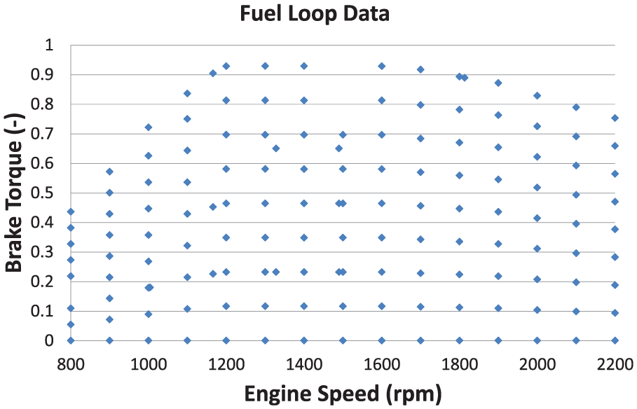
Fuel loop is a naming convention used in dynamometer testing. A fuel loop test is executed via collecting data at engine speed and load values spanning the full operation range (0%–100%). In this study, three different fuel loop data are gathered in dynamometer tests.

The main goal is to collect sufficient data covering different feed gas NO_x levels for methodology generation and validation. It is aimed to investigate the accuracy of the methodology with the same hardware and at same engine speed and torque values, but at different operating conditions such as air flow, boost pressure, turbine inlet temperature and hence different emission outputs. Collecting the fuel loop data at different boost temperature values specifically served to this purpose. Table 2 shows the boost temperature of the three different fuel loop data sets that are measured in the dynamometer tests. In each of these three experiments, data are collected at 140 different operating points corresponding to 10% intervals of engine load at different speeds. Figure 1 shows the operating points used in the measurements of fuel loops.

Table 2.

Fuel loop data sets.

	Boost temperature	Number of points
Fuel Loop 1	30 °C	140
Fuel Loop 2	40 °C	140
Fuel Loop 3	50 °C	140

Figure 1.

Fuel loop points.

Fuel Loop 1 is used for model correlation. Figures 2–6 show the comparison between model predictions and the test measurements under full load conditions.

Figure 2.

Full load correlation comparison: (a) BMEP,(b) GMEP and (c) PMEP.

Figure 3.

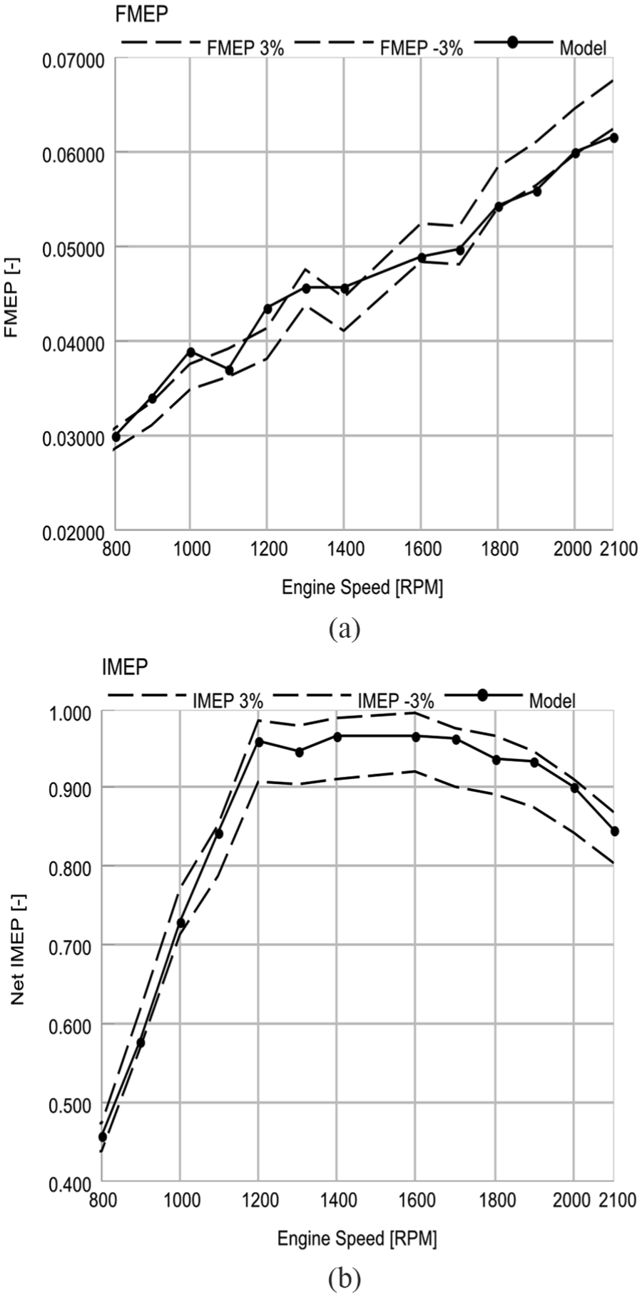
Full load correlation comparison: (a) FMEP and(b) IMEP.

Figure 4.

Full load correlation comparison – compressor results: (a) compressor outlet pressure and (b) compressor outlet temperature.

Figure 5.

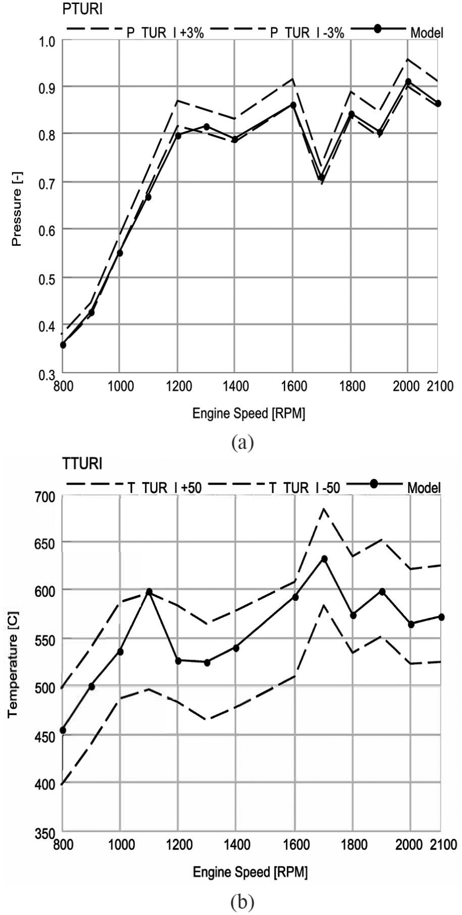
Full load correlation comparison – turbine results: (a) turbine inlet temperature and (b) turbine inlet pressure.

Figure 6.

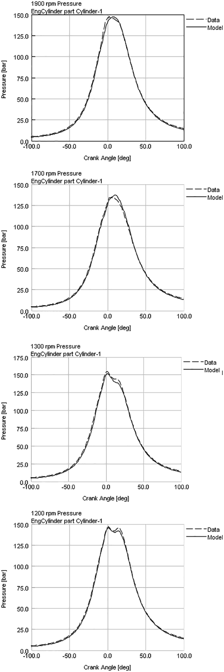
In-cylinder pressure curve comparisons at different operating points.

Figures 2 and 3 show that indicated mean effective pressure (IMEP), GMEP, BMEP, pumping mean effective pressure (PMEP) and friction mean effective pressure (FMEP) are mostly within ±3% accuracy band indicating that accuracy of combustion and friction models is quite good. The main contribution for PMEP is the difference between turbine inlet pressure and boost pressure. Increase in this difference results in an increase in the pumping losses. In this study, the fuel loop correlation was performed with high accuracy in both turbine inlet pressure and boost pressure. Hence, for any operating condition, the thermodynamic model calculates the pumping losses accurately.

Generally, thermodynamical models need some efficiency or mass flow multipliers to ensure a good correlation of compressor outlet temperature and turbine inlet pressure values. This is mainly a result of miscalculated heat transfer or ignored friction values during turbocharger map generation in a turbocharger test bench. To keep the model outputs in alignment with dynamometer test bench data, efficiency multipliers (located in the thermodynamic model’s turbocharger objects) can be used. Figure 4 shows that compressor outlet pressure and compressor outlet temperature values lay within the acceptable ±3% and ±10°C accuracy bands, respectively. Figure 5 shows that turbine inlet pressure and turbine inlet temperature values are also within the acceptable ±3% and ±50°C accuracy bands, respectively. In this study, use of such efficiency multipliers is not needed, and compressor and turbine maps successfully cover the real test conditions, including heat transfer, friction, and so on.

Figure 6 shows that model in-cylinder pressure values are in good correlation with test data. The peak firing pressure outputs of the model are mostly within ±2.5 bar difference range.

Figure 7 shows NO_x emission measurements for three different fuel loops. Non-dimensional contour plots are generated by dividing the measured values by the maximum NO_x measured value. HORIBA PG-250 multi-gas portable analyzer is used to gather NO_x emission data. Technical specification of the device shows that the measurement accuracy for NO emission is ±1%. Fuel Loop 3, which is the loop with the highest boost temperature, shows the highest NO_x emissions. Maximum NO_x values are met near the full load range, especially in the 1200–1600 r/min range in all of these fuel loops.

Figure 7.

NO_x emission comparison of different fuel loops.

NO_x model and calibration

In the proposed method, the NO_x emissions are calculated using the extended Zeldovich mechanism embedded in the GT-Suite-based thermodynamical model. Table 3 shows the reactions representing the extended Zeldovich mechanism and their rate equations. All reactions are two-way reactions and the rates shown are the forward reaction rates. Use of equilibrium constant and the forward rate gives the reverse reaction rates. To tune the model NO_x emission outputs to experimental data, it is possible to employ a calibration multiplier which modifies the net rate of formation.

Table 3.

Extended Zeldovich mechanism reactions.

Reaction	Forward reaction rate $({\mathrm{m}}^3\mathrm{g}\mathrm{mo}{\mathrm{l}}^{-1}{\mathrm{s}}^{-1})$
N2 + O = NO+N	$k_1=1.8\times {10}^8{e}^{-38,370/T}$
N + O2 = NO+O	$k_2=1.8\times {10}^{4}T{e}^{-4680/T}$
N + OH = NO+H	$k_3=7.1\times {10}^{7}T{e}^{-450/T}$

Once the model runs with Fuel Loop 1 inputs, NO_x outputs of the model are compared with test data. The ratio between the model NO_x and dynamometer NO_x values is called calibration multiplier. To enhance the model’s NO_x prediction accuracy, these multipliers can be utilized via generating suitable multidimensional look-up tables. The inputs of these multidimensional look-up tables are different engine performance parameters such as turbine inlet temperature, injected fuel quantity and engine speed. The only output is the NO_x calibration multiplier. Utilizing the ‘Multidimensional Table Look-up Using Scattered Data’ object embedded into GT-Suite, it is possible to generate and use different maps providing NO_x calibration multipliers. Use of these maps enables accurate NO_x prediction with low computational resources. For example, it is possible to generate the NO_x prediction for 100 points within only 30 min on a PC with i7 CPU.

In the below studies, the aim is to find out the best engine performance parameters to be used for map generation. Hence, emission model is correlated by calculating the calibration multipliers that provide ±2% accuracy in comparison with experimental results for each point in Fuel Loop 1.

Once the NO_x calibration multipliers generated using Fuel Loop 1 and mapped via different engine performance parameters, Fuel Loops 2 and 3 are run to see the NO_x prediction accuracy of the generated maps. These two fuel loops are used for measuring the prediction capability of the different maps only, and they are not used for map generation. Errors in NO_x predictions are calculated via the equation below

$$\mathrm{Error}(\mathrm{\%})=100\frac{\mathrm{N}{\mathrm{O}}_{\mathrm{x},\mathrm{model}}-\mathrm{N}{\mathrm{O}}_{\mathrm{x},\mathrm{test}}}{\mathrm{N}{\mathrm{O}}_{\mathrm{x},\mathrm{test}}}$$

(1)

Also, non-dimensional root mean square error (nRMSE) values are calculated via below equations

$$\mathrm{RMSE}(\mathrm{ppm})=\sqrt{\frac{1}{n}\sum _{i=1}^n{(\mathrm{N}{\mathrm{O}}_{\mathrm{x},\mathrm{test}}-\mathrm{N}{\mathrm{O}}_{\mathrm{x},\mathrm{model}})}^2}$$

(2)

$$\mathrm{nRMSE}(\mathrm{\%})=100\frac{\mathrm{RMSE}}{\mathrm{N}{\mathrm{O}}_{\mathrm{x},\max }-\mathrm{N}{\mathrm{O}}_{\mathrm{x},\min }}$$

(3)

The main steps of the correlation methodology can be summarized as follows:

1. Generate engine model using 3D CAD geometry, valve lifts, discharge coefficients, and so on.

2. Perform fuel loop correlation of engine model to test data.

3. Compare the model NO_x output and corresponding dynamometer data to calculate NO_x calibration multipliers for each case.

4. Generate maps of NO_x calibration multipliers using different engine performance parameters as inputs.

5. Use other test data to evaluate the effectiveness of the generated maps. Compare the results of different maps regarding emission prediction accuracy.

6. Select the map with the highest accuracy.

It is shown in this study that these methodological steps are valid independently of the engine volume and power. One can use the same steps with a different engine, as well.

NO_x calibration multiplier maps

To enhance the NO_x prediction accuracy of the model, selection of proper map parameters has critical importance. Various parameters such as engine speed, load and EGR flow rate are used for NO_x calibration multiplier map generation utilizing data of Fuel Loop 1. This section includes the selection of input parameters used for the map generation and the resulting NO_x emission prediction accuracy obtained for Fuel Loops 2 and 3.

Independent variables such as test injection pressure, pilot- and post-injection timing and quantities are not used as primary inputs since these parameters are not variables of Diesel Wiebe; the current combustion model. Air mass flow rate target (to define EGR rate), boost pressure and temperature, injected total fuel quantity, engine speed and maximum in-cylinder pressure values are the prime inputs in models including Diesel Wiebe combustion model. Utilizing injection pressure, pilot- and post-injection timing and quantities as direct inputs requires the use of a predictive combustion tool, like DI-Pulse. However, in DI-Pulse, user needs detailed information (such as injector pulse widths) which is generally confidential for injector suppliers. In this article, the methodology is generated without any need for such kind of data. Heat release rates which are generated using Diesel Wiebe include the effect of these parameters.

Fifteen different maps are generated by the use of 11 different parameters, which are engine speed (RPM), engine load (Load), calculated EGR flow rate, turbine inlet temperature (TTURBI), in-cylinder maximum pressure (Pmax), in-cylinder maximum temperature (Tmax), fuel flow rate, CA50, fuel–air ratio, EGR rate and rail pressure.

Engine speed is selected as the first parameter since it mainly represents the air flow capability, friction and pumping losses which indirectly effect the NO_x emission formation. Besides, in the literature, there are many studies using engine speed parameter for NO_x emission prediction.^25–27 EGR flow is also chosen since it is one of the main parameters showing a significant trend on NO_x formation.

Hence, engine speed and the EGR flow parameters are selected as the initial input parameters used in the production of the first NO_x calibration multiplier map. Once the map is created with the outputs of Fuel Loop 1, Fuel Loops 2 and 3 are run with this map to see the NO_x prediction capability. Results are shown in Figure 8; 29% of total points are between 0 and 25 ppm delta error band, and 47% of total points are between 0% and 15% error band. nRMSE is approximately 17%.

Figure 8.

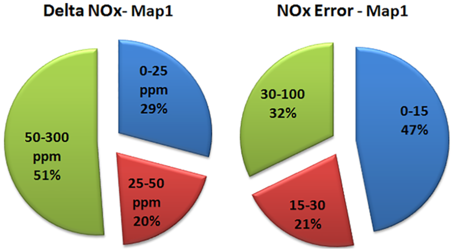
Model versus test data: MAP1 = f(RPM, EGR Flow).

It seems that the EGR flow parameter does not show the expected trend for NO_x prediction. One possible reason is the lack of EGR flow measurements in dynamometer tests. Since experimentally measured EGR flow data are not available, the values are generated via thermodynamic model. Air mass flow rate values are targeted and EGR valve position is changed to reach the targeted air mass flow rates. So, EGR flow values calculated from the thermodynamic model may represent significant differences with respect to actual values. That may also be the explanation about the slight change in NO_x prediction of MAP9 with respect to MAP8, which will be mentioned below.

In the second map, load is also considered as an input parameter. Load represents the operating condition of an engine at certain engine speed. Like engine speed parameter, load is also selected as the main input of emission-based prediction neural networks in many studies.^25,28 This is because it directly represents all of the operating variables of an engine, not only injected flow, SOI and so on but also friction and pumping losses, as well.

As Figure 9 shows, 30% of total points lay between 0 and 25 ppm delta error band, and 49% of total points lay between 0% and 15% error band. Although the use of the engine load as an additional input gave slightly better results, the map is not still sufficiently accurate. nRMSE of this map is approximately 14%.

Figure 9.

Model versus test data: MAP2 = f(RPM, Load, EGR Flow).

Since NO_x emissions are the primary function of in-cylinder temperature and combustion characteristics, it is decided to use turbine inlet temperature as one of the inputs for the map generation. The turbine inlet temperature is very important in engine combustion. It mainly depends on fuel–air equivalence ratio, injection timing and engine speed. All these parameters have significant effects on combustion. Generally, at the same operating point, higher efficiency results in lower turbine inlet temperature and higher NO_x formation. On the contrary, lower efficiency results in higher turbine inlet temperature and lower NO_x formation. Turbine inlet temperature, engine load and EGR flow rate are parameters for the third map. Figure 10 shows that this map did only provide a small difference in the accuracy of the predictions, and nRMSE, which is 21%, is still too high.

Figure 10.

Model versus test data: MAP3 = f(TTURBI, Load, EGR Flow).

In the fourth map, maximum in-cylinder pressure, in other words, peak firing pressure (PFP) is added to the previous map. It is known that the maximum in-cylinder pressure value is an essential result of thein-cylinder combustion. The maximum value of in-cylinder pressure has great importance and effect on in-cylinder maximum temperature values and hence on NO_x emissions. Combustion at higher speed results in higher in-cylinder maximum temperature and pressure values. Higher in-cylinder temperature values mostly result in higher NO_x formation. At the same operating point, lower maximum in-cylinder pressure values are encountered as a result of retarded combustion, which means lower in-cylinder maximum pressure and temperature and higher exhaust temperature. So, like in-cylinder maximum temperature, in-cylinder maximum pressure values can also be selected for a better NO_x prediction.

As a result of the fourth map, 35% of total points lay between 0 and 25 ppm delta error band, and 55% of total points lay between 0% and 15% error bands. Hence, almost 5% enhancement is obtained on both delta and percentage differences. nRMSE of this map is better than the previous one: 19%.

A fifth map is generated via employing turbine inlet temperature and engine load, only to understand the particular impact of PFP. Accuracy is lowered for this map proving that PFP is an important parameter for NO_x prediction. nRMSE remains almost the same: 19%.

The sixth map includes turbine inlet temperature and maximum in-cylinder temperature parameters. In this map, the effect of maximum in-cylinder temperature is investigated. It is obvious that there is a strong correlation between in-cylinder maximum temperature and NO_x formation. In-cylinder maximum temperature is a significant parameter on NO_x prediction since higher in-cylinder maximum temperature values result in higher NO_x formation. Although in dynamometer tests, it is generally not possible or very expensive to collect in-cylinder maximum temperature values, but with a correlated thermodynamic model, it is possible to calculate it and use for NO_x emission prediction.

It is found that some NO_x calibration multipliers remain at very high values (approximately 7–10). As a result, these relatively large values are reducing the interpolation accuracy at the neighbour load–speed points. These high-calibration multipliers, which are so-called outliers, are calculated at points where dynamometer test values are more than three times of model NO_x values. The number of these points is very low (approximately 1.5% of total map points) and their values are much different than their neighbouring points. Since there is no trend about the physical condition, these outliers are most probably encountered as a result of measurement errors (such as HORIBA device or measurement duration related) in the dynamometer tests. In the mapping process, these outliers are eliminated to increase the accuracy.

It is essential to note that the same investigation is performed for the previous maps as well. However, the effect of outliers was not as decisive as they are in this case. So, outliers were not eliminated in the earlier maps.

Although the sixth map only includes turbine inlet temperature and maximum in-cylinder temperature values, better accuracy with respect to previous maps is obtained. As it is seen in Figure 11, 33% of total points lay between 0 and 25 ppm delta error band, and 57% of total points lay between 0% and 15% error band. nRMSE is significantly improved: 7.6%. This result shows that the in-cylinder maximum temperature has critical importance for emission prediction.

Figure 11.

Model versus test data: MAP6 = f(TTURBI, Tmax).

Since the main contributors of the NO_x emissions are in-cylinder temperature and pressure values, the seventh map is generated based on these two parameters and turbine inlet temperature. It is found that 39% of total points lay between 0 and 25 ppm delta error band and 60% of total points lay between 0% and 15% error band. nRMSE slightly increases: 8.6%.

The load parameter is added to MAP7 parameters to generate MAP8. It is found that adding load parameter for mapping has a slight improvement on NO_x emission prediction. Accuracy is enhanced, and nRMSE decreases in comparison with the previous map: 7.8%.

EGR flow parameter is added to MAP9 to enhance the accuracy. However, a slight decrease in accuracy is encountered. This is mainly because of non-linearity of EGR flow values and calculation errors encountered in the dynamometer test. nRMSE slightly decreases to 8.9%.

Hence, it is decided to eliminate the EGR flow from the map and introduce fuel flow rate to increase the accuracy. Similar to the load parameter, injected total fuel quantity is a direct representative of CO₂ emission. Injected total fuel quantity is also defining the air–fuel ratio for constant air mass flow rate, and it directly affects the combustion. As a result of higher injected fuel quantity, higher engine operating loads are obtained at a particular engine speed, resulting in higher NO_x emissions.

As it is seen in Figure 12, 52% of total points lay between 0 and 25 ppm delta error band, and 74% of total points lay between 0% and 15% error band. These results show that these five parameters – turbine inlet temperature, in-cylinder maximum pressure, in-cylinder maximum temperature, engine load and total injected fuel mass flow – are the main parameters to be used for NO_x prediction. nRMSE of this map is the best among all, which is 5.7%.

Figure 12.

Model versus test data: MAP10 = f(TTURBI, Tmax, Pmax, Load, Fuel Flow).

General trends of the model and test outputs can also be seen in Figure 13. The ordinate is representing the non-dimensional NO_x data. As it is seen in this regression graph, model outputs seem to be in good correlation with dynamometer test results.

Figure 13.

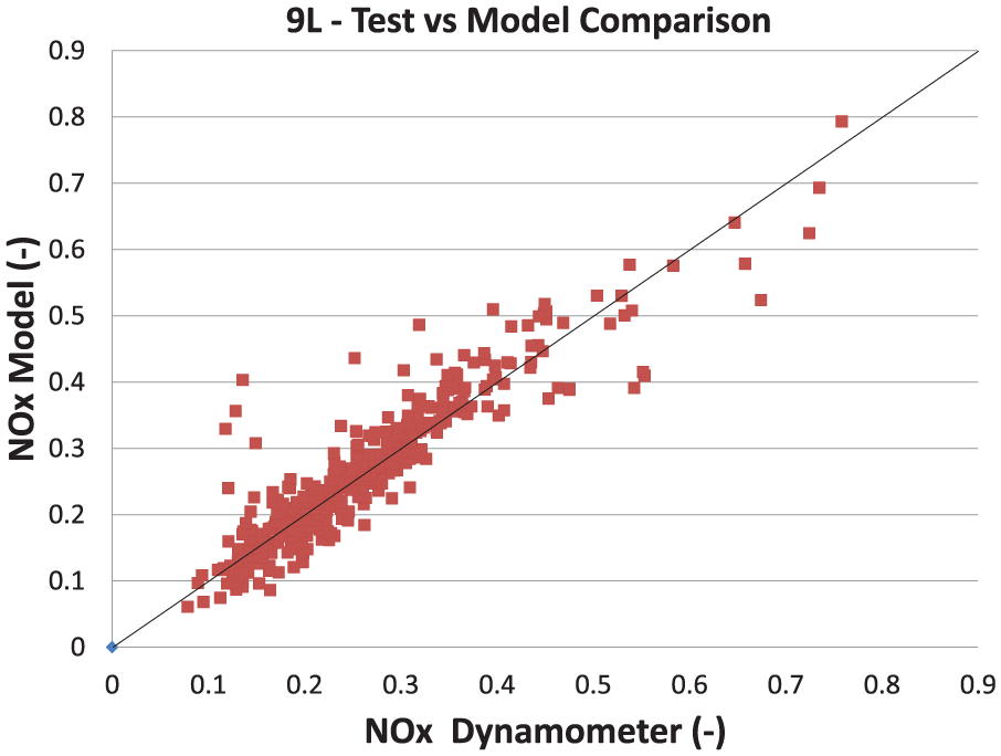
Model versus test data–Regression chart of Map10.

Effect of CA50 parameter is taken into account in MAP11. In this map, the turbine inlet temperature parameter is replaced with CA50 since it shows the combustion location and represents the premixed phase characteristics. It is found that the nRMSE is 5.8%, which is similar to the MAP10 results. This result has proven that the CA50 can also be used for the NO_x emission prediction.

It is obvious that the fuel flow parameter used in MAP10 is not a normalized parameter and may lead to some troubles when trying to generalize the model. Instead, it is replaced by the fuel–air equivalence ratio in MAP12, which is linked to the fuel flow, but expressed in a normalized way. This would have a clear advantage when trying to generalize the model (i.e. to use the same already calibrated model for another engine). nRMSE value of this map is 6.2%.

In the previous maps, EGR flow was directly used. However, EGR rate may be a better NO_x emission prediction parameter; since in reality, EGR rate is the most significant parameter that can be used for NO_x control. EGR rate is calculated in the engine model via equation (4)

$$\mathrm{EGR}\mathrm{rate}(\mathrm{\%})=100\frac{\mathrm{EGR}\mathrm{Flow}}{\mathrm{EGR}\mathrm{Flow}+\mathrm{Air}\mathrm{Mass}\mathrm{Flow}}$$

(4)

MAP13 includes CA50, in-cylinder maximum temperature, load, fuel–air equivalence ratio and EGR rate as parameters. nRMSE value of this map is 7.2%, which shows that using the model EGR rate output as a map parameter provides acceptable NO_x prediction accuracy.

As the last parameter, the rail pressure is investigated. The rail pressure is an input quantity in the engine tests. As it was mentioned previously, the current combustion model cannot use the rail pressure parameter as an input. In other words, model outputs do not change when different rail pressure values are imposed to the model. But its use as an NO_x emission prediction parameter is still possible within the scope of this methodology. To do this, the rail pressure data collected from Fuel Loop 1 are used as a parameter in MAP14. The map also includes CA50, in-cylinder maximum temperature, load and fuel–air equivalence ratio parameters. Model is run with Fuel Loops 2 and 3 set points, also including the rail pressure values collected from test data. nRMSE value of this map is 6.1%. This result shows the importance of the rail pressure parameter in NO_x prediction.

In the last map, CA50, in-cylinder maximum temperature, EGR rate, rail pressure and fuel–air equivalence ratio parameters are used. nRMSE value of this map is 6.6%.

All of the maps and their parameters are listed in Table 4. In Figure 14, accuracy values of different maps are shown. nRMSE comparison of different maps is shown in Figure 15. MAP10–MAP15 generate the best nRMSE values. This condition shows that turbine inlet temperature, maximum in-cylinder temperature, maximum in-cylinder pressure, load, fuel flow, CA50, fuel–air equivalence ratio, EGR rate and rail pressure parameters are the most critical emission prediction parameters. Among these parameters, it is known that EGR rate and rail pressure are some of the most important parameters for NO_x emission control during engine calibration.

Table 4.

Maps and parameters.

MAP1	f(RPM, EGR Flow)
MAP2	f(RPM, Load, EGR Flow)
MAP3	f(TTURBI, Load, EGR Flow)
MAP4	f(TTURBI, Load, EGR Flow, Pmax)
MAP5	f(TTURBI, Load)
MAP6	f(TTURBI, Tmax) Without Outliers
MAP7	f(TTURBI, Tmax, Pmax)
MAP8	f(TTURBI, Tmax, Pmax, Load)
MAP9	f(TTURBI, Tmax, Pmax, Load, EGR Flow)
MAP10	f(TTURBI, Tmax, Pmax, Load, Fuel Flow)
MAP11	f(CA50, Tmax, Pmax, Load, Fuel Flow)
MAP12	f(TTURBI, Tmax, Pmax, Load, Fuel-Air Ratio)
MAP13	f(CA50, Tmax, EGR Rate, Load, Fuel-Air Ratio)
MAP14	f(CA50, Tmax, Rail Pressure, Load, Fuel-Air Ratio)
MAP15	f(CA50, Tmax, EGR Rate, Rail Pressure,Fuel-Air Ratio)

Figure 14.

Model versus test data of 12 different maps.

Figure 15.

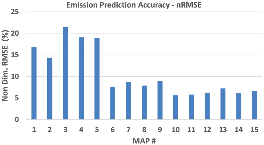
Non-dimensional RMSE values of 12 different maps.

Methodology results in a different engine

For a further understanding of the effectiveness of the methodology, another heavy-duty engine is used. Important parameters for the chosen engine are as listed in Table 5. This table shows the main aspects of the heavy-duty diesel engine used for the methodology trial.

Table 5.

12.7L Heavy-duty diesel engine specifications.

Volume	12.7 L
Maximum power	480 PS
Compression ratio	16.5:1
Bore	160 mm
Stroke	215 mm
Number of cylinders	6
Injection system	Common rail
Injection system pressure	2500 bar

First of all, as it was performed in the 9-L engine studies, fuel loop data correlation is performed. Brake power, brake torque, air–fuel ratio, air mass flow and fuel mass flow values have good correlation with dynamometer test data.

The developed methodology is performed with the same steps after completing the correlation. A fuel loop data set with 173 points in total is used for this study. In all, 33% (56 points) are used for NO_x calibration multiplier multidimensional look-up table generation, and the remaining 67% (117 points) are kept for methodology examination.

Figure 16 illustrates that dynamometer data and model results have quite good correlation, which is even better than the 9-L engine comparison. Besides, non-dimensional RMSE value, in this case, is 5.1%. These results are showing that the methodology can be used for different engines with different volumes successfully. This is mainly because the two engines are both representing heavy-duty diesel characteristics.

Figure 16.

Model versus test data – regression chart.

The methodological steps represented in this study apply to all heavy-duty diesel engine variants with different cylinder volume or power. As it was summarized above, using the methodological steps developed in this study, it is possible to find out most effective parameters on feed gas NO_x formation once the thermodynamical model is created and correlated with test data.

For the case that an entirely new concept engine will be developed, NO_x prediction maps generated with similar engine properties (displacement, power, torque, etc.) may be used. But, the accuracy of the methodology most probably would be lower due to the lack of actual test data for model correlation. However, the necessary data for method application may be generated from a few 3D CFD simulations or single-cylinder engine tests at very early stages of engine development when an actual engine does not exist. Hence, it would be possible to direct hardware selection studies by considering the NO_x emission outputs.

Conclusion

In this study, an agile methodology valid for NO_x emission prediction at all stages of engine development is developed. A 9-L 380-PS heavy-duty diesel engine model is generated and correlated with fuel loop data, which include whole engine speed range with 10% load increments.

Extended Zeldovich mechanism is used in GT-Suite for NO_x emission calculation. NO_x emission output correlation with test data is completed using NO_x calibration multiplier maps. Most critical parameters in NO_x emission prediction with high accuracy are investigated. Fifteen different maps are generated, and model NO_x outputs are compared with two separate fuel loop data.

Results show that in-cylinder maximum pressure and in-cylinder maximum temperature are the most critical parameters for NO_x emission prediction. Turbine inlet temperature, engine load, fuel flow, CA50, EGR rate and fuel–air ratio are the other important parameters that can be used for generating NO_x calibration multiplier maps.

Furthermore, to understand the robustness of the developed methodology, another heavy-duty engine data are also used. A 12.7-L heavy-duty diesel engine model is created, and model correlation is performed using fuel loop test data. Same methodological steps are accomplished, and better accuracy in NO_x emission prediction is obtained. In the 12.7-L diesel engine study, nRMSE value between dynamometer and model NO_x outputs is 5.1%, which is better than 9-L diesel engine correlation: 5.7%. It seems that the accuracy level of the developed methodology is competitive with the other NO_x emission prediction modelling strategies mentioned previously in the ‘NO_x emission models’ section.

Hence, this study has shown that if the minimum data requirement is satisfied via dynamometer tests, global optimization can be done in the simulation environment without any further tests. Furthermore, since thermodynamical models are physically based, the demonstrated methodology can be used at the very early stages of engine development, in which no actual engine or test data exist. Undoubtedly, this will provide both cheaper and faster solution for global optimization and component selection studies.

Last but not least, traditional emission prediction methodologies require significantly high simulation duration (almost 3–4 days per operating point on a typical workstation PC). However, this methodology enables accurate NO_x prediction with very low CPU time. For example, it is possible to generate the NO_x prediction for 100 points in 30 min. Using a single-cylinder thermodynamical model rather than a detailed model (six cylinders) may even further decrease the required computational effort. Taking the points that are mentioned above into consideration, it is possible to state that the methodology presented in this article can be used as a fast and reliable tool for NO_x prediction at any phase of engine development.