Sage Journals: Discover world-class research

Abstract

In order to improve the effect of estimating travel time and provide more precise and reliable traffic information to traffic management department and travelers, we proposed an arterial travel time estimation method using Sydney Coordinated Adaptive Traffic System traffic data based on K-nearest neighbor–least squares support vector regression model. First, the virtual time series is constructed by analyzing the characteristics of the inconsistent time intervals of Sydney Coordinated Adaptive Traffic System traffic data. Second, the K-nearest neighbor method was used to search the K similarity patterns matching the current traffic pattern and obtain K travel time data. Then, the least squares support vector regression model was used to perform travel time estimation. Finally, case validation is carried out using the measured data of Sydney Coordinated Adaptive Traffic System traffic control system. The estimation results demonstrate that the travel time estimation accuracy of proposed method outperforms the other two methods.

Keywords

Arterial travel time estimation Sydney Coordinated Adaptive Traffic System traffic data virtual time series K-nearest neighbor search mechanism least squares support vector regression model

Introduction

Travel time is an important measurement for evaluating the performance of traffic management strategies.¹ From the traffic manager’s point of view, they could make full use of the travel time information to balance travel demand in different parts of a road network and achieve more efficient use of existing traffic infrastructure. From the traveler’s perspective, accurate time information helps them to make better decisions in terms of route selection or mode choice, and when given pre-trip it allows them to choose the time of departure, thus alleviating driver stress. Research has illustrated that about 77.7% drivers will change their travel route based on travel time information and even if there is no any alternative route, they will find driving less stressful when knowing what to expect ahead of them.² However, it is well known that travel time estimation is not an easy task because travel time is a complex dynamic parameter which is influenced by a range of different factors, such as driver characteristics, weather conditions, traffic flow characteristics, road way conditions, and so on. In particular, the travel time estimation for arterial is a more challenging task because arterials are interrupted facilities with traffic signals and other control devices. Therefore, the travel time estimation, especially for arterial, has been recognized as a critical need for the intelligent transportation systems.

At present, the methods for collecting travel time data can be generally divided into two categories. The first category is direct approaches which use automatic vehicle identification data,^3,4 probe vehicles data,^5–8 toll collection system data,^9,10 and mobile phones data.^11–13 Travel time data can be quickly collected via these approaches, but most of the direct travel time measurement techniques are expensive and immature. The second category of methods for collecting travel time data is indirect approach in which loop detectors are the most commonly used equipment.^14–17 Currently, the indirect travel time estimation methods can be generally divided into four classes: speed-based estimation models,^18,19 cumulative plot-based methods,²⁰ regression models,^21,22 and artificial intelligence methods.^23–25 Li et al.¹⁸ compared the performance of four speed-based travel time estimation methods: an instantaneous model, a time slice model, a dynamic time slice model, and a linear model. Van Lint and van der Zijpp¹⁹ presented a new travel time estimation algorithm based on a linear function of speed. Bhaskar et al.²⁰ presented a travel time estimation method based on cumulative plots for urban signalized intersections. Kwon et al.²¹ formulated their regression model using flow, occupancy, time of departure, and day of week. Tang et al.²³ designed a new travel time estimator based on an evolving fuzzy neural network by using traffic flow data collected from existing loop detectors. Liu et al.²⁴ presented a neural network–based traffic flow model to estimate urban arterial travel time.

Travel time estimation has generated great interest among researchers and a significant number of methods exist in the literature. However, due to the special location of vehicle detectors and the special data types in the Sydney Coordinated Adaptive Traffic System (SCATS) traffic control system, there are few related research results. Luk et al.²⁶ described the ARRB travel time model for estimating arterial travel times for general traffic and buses. The model retrieves traffic data from SCATS each minute and has been implemented in a server at VicRoads. Mazloumi et al.²⁷ presented an artificial neural network that used saturation degree data collected by the SCATS at intermediate signalized intersections along with schedule adherence to predict bus travel time. Cheu et al.²⁸ introduced a model to estimate average link travel time of signalized arterials using data obtained from detectors in SCATS. The related studies often assumed that vehicle detectors can obtain traffic data according to certain fixed sampling intervals, even on the basis of some data that are not available at present. These assumptions do not conform to the actual situation of SCATS traffic control system. Jiang et al.²⁹ designed a travel time estimation method using SCATS data based on k-NN algorithm, but this method only considered the linear relationship of travel time data, the accuracy of travel time estimation needs to be further improved. Taking into account the above reasons, and with the goal of improving the accuracy of travel time estimation for arterial, we put forward arterial travel time estimation method using SCATS traffic data based on K-nearest neighbor (KNN)–least squares support vector regression (LSSVR) model. The remainder of this article is structured as follows: Section “Feature analysis and processing of SCATS data” presents the feature analysis and processing of SCATS data. Section “Arterial travel time estimation based on KNN-LSSVM model” gives the arterial travel time estimation based on KNN-LSSVR model. Section “Empirical analysis” describes the empirical analysis. Section “Conclusion” draws some conclusions.

Feature analysis and processing of SCATS data

Characteristics analysis of SCATS traffic data

SCATS traffic control system employs 16–32 loop detectors per intersection to obtain traffic parameter data. The large quantity of detectors is located downstream of lane and near stop line which could record traffic information per signal cycle. The traffic information recorded by the SCATS system is shown in Table 1.

Table 1.

The traffic information recorded by the SCATS system.

Detector number	Signalphase	Starttime	Greentimes (s)	Cyclelength (s)	DS values (%)	Time headway (s)	Traffic counts (veh)
08081210	A	2009-5-25 0:00:12	54	103	26	9	5
08081203	B	2009-5-25 0:01:06	18	103	35	9	2
08081211	C	2009-5-25 0:01: 24	31	103	13	15.5	2

SCATS: Sydney Coordinated Adaptive Traffic System.

As we can see from Table 1, the SCATS traffic control system can provide two kinds of traffic information. One is the signal setting information such as cycle length, signal phase, start time of per phase, and green times. The other is traffic parameter information such as traffic counts and time headway during each phase green time.

Through extensive analysis of the basic data obtained from the SCATS traffic control system, the following main characteristics were found:

The traffic parameters provided by the SCATS traffic control system include traffic counts and average headway time, not providing speed and occupancy data.

The detectors of SCATS traffic control system are placed in front of the stop line of the intersection. Therefore, the obtained traffic parameter data can’t reflect the influence of different number of queued vehicles on the road, which will limit the application of data to a certain extent.

The data sampling interval of SCATS traffic control system is determined by green signal phase, while the green phase duration is dynamically changing. Therefore, the traffic parameter data of each sampling interval are not strictly comparable, which increases the difficulty of travel time estimation.

Construction of virtual time series for SCATS traffic data

In order to obtain the data time series of the SCATS traffic control system with a fixed sampling interval, this article proposes the concept of a virtual time series. The basic principle is that the arrival of the vehicle in each signal cycle converts from random distribution to uniform distribution. A virtual sampling interval (5 min, 10 min, etc.) is set up and inserted into the time axis of SCATS traffic control system data. The actual sampling interval of the SCATS traffic control system is still the green signal phase, while the virtual sampling interval is the setting time length. The traffic data in each virtual sampling interval can be obtained by converting the corresponding data in the actual sampling interval. Schematic diagram of virtual sampling interval interpolation is shown as Figure 1, where C represents different signal cycle and $τ$ represents virtual time interval.

1. Conversion of traffic flow during virtual sampling interval.

Figure 1.

Schematic diagram of virtual sampling interval interpolation.

Traffic flow is a cumulative value. Under the assumption that the vehicle is uniformly arriving, the number of vehicles arriving per unit time in a signal cycle is equal to the ratio of the actual number of vehicles arriving to the signal cycle length, which is called the average traffic flow

{\bar{q}}_{i, s} = \frac{q_{i, s}}{C_{i, s}}

(1)

where ${\bar{q}}_{i, s}$ is the average traffic flow within the actual sampling interval, q_i,s is the actual number of vehicles arriving, and C_i,s is the signal cycle length.

The traffic flow mapping relationship from the actual sampling interval to the virtual sampling interval is as follows

q_{j, x} = \sum_{n = i}^{i + N} {\bar{q}}_{i, s} \times t_{i}

(2)

where q_j,x is the traffic flow within the virtual sampling interval, t_i is the part time length of the virtual sampling interval j located in the actual sampling interval i, and N is the number of jth virtual sampling interval spanning the actual sampling interval.

2. Conversion of average time headway during virtual sampling interval.

Under the actual sampling interval, the average time headway is the average time interval between random arrival vehicles, which is equivalent to converting the vehicle arrival mode from the random distribution to the uniform distribution. Therefore, at the virtual sampling interval, the calculation of the average headway time is as follows

h_{j, x} = \frac{\sum_{n = i}^{i + N} (h_{i, s} \times t_{i} \times {\bar{q}}_{i, s})}{\sum_{n = i}^{i + N} (t_{i} \times {\bar{q}}_{i, s})}

(3)

where h_j,x is the average time headway of the virtual sampling interval, and h_i,s is the average time headway of the actual sampling interval i.

3. Conversion of traffic signal control parameters during virtual sampling interval.

SCATS traffic control system adopts the small-step online selection method to dynamically optimize the timing parameters. The difference of the adjacent signal cycle is within 6 s, which is shown as Figure 2.

Figure 2.

Schematic of green time and cycle time.

Therefore, in the virtual sampling interval j, the cycle length and the green times can be approximated as the average of the corresponding parameters of the actual sampling interval i. The specific mapping relationship is as follows

g_{j, x} = \sum_{n = i}^{i + N} \frac{g_{i, s}}{N}

(4)

C_{j, x} = \sum_{n = i}^{i + N} \frac{C_{i, s}}{N}

(5)

where g_j,x and C_j,x are the average green times and average cycle length of the virtual sampling interval j, respectively, and g_i,s is the green times of the actual sampling interval i.

In the SCATS traffic control system, saturation refers to the ratio of the effective green time to the green time. The mapping relationship from the actual sampling interval i to the virtual sampling interval j is as follows

D S_{j, x} = \frac{\sum_{n = i}^{i + N} D S_{i, s} \times g_{i, s}}{\sum_{n = i}^{i + N} g_{i, s}}

(6)

where DS_j,x is the average saturation of the virtual sampling interval j, and DS_i,s is the saturation of the actual sampling interval i.

Arterial travel time estimation based on KNN-LSSVM model

KNN search mechanism

The KNN algorithm is based on the pattern recognition theory. The premise is that the current pattern of the research object has similarities with several historical pattern. The basic principle is to search for the most K similar historical patterns to the current pattern in the specified database and determining the pattern similarity measure method. Based on this, the target travel time value corresponding to the current traffic pattern is obtained. The traffic parameter data have both stochastic volatility and long-term trend, so it can meet the needs of KNN algorithm to a certain extent.

1. The definition of the feature vector.

Feature vectors are the criteria for comparing current traffic patterns with historical traffic patterns. There is no uniform standard for the selection of feature vectors. Taking as many factors as possible into the feature vector not only does not improve the estimation accuracy but also can increase the running time of the algorithm. Therefore, this article will determine the appropriate feature vector composition based on the characteristics of SCATS traffic data.

2. Selection of similarity measure method.

At present, multiple similarity measure methods can be applied to KNN search, such as Chebyshev distance, Mahalanobis distance, Euclidean distance, and so on. It has been proved that the use of different spatial distance measures does not have a significant impact on the final outcome of the research object.³⁰ Therefore, this article will calculate the Euclidean distance of the feature vector between the current traffic pattern and the historical traffic pattern, which is used to measure the matching degree between different traffic patterns

d_{i} = \sqrt{\sum_{i = 1}^{n} {(V_{i} - {\hat{V}}_{i})}^{2}}

(7)

where d_i is the distance between current data and ith group data in the historical database, V_i is the value of the ith item in the current data, ${\hat{V}}_{i}$ is the value of the ith item in the historical database, and n is the number of items in the feature vector.

3. The determination of the nearest neighbor number K.

The selection of K value is largely related to the specific situation of historical data and the specific composition of feature vectors. At present, there are no rules to guide the selection of K value. In this article, aiming at the specific experimental environment, the determination of the K value is based on the minimum error of the estimated travel time.

The principle of LSSVR model

LSSVR is an improved algorithm based on SVR. By introducing the method of equality constraint and least square loss function, the optimization problem is changed into a linear equation, and the complexity of the algorithm is reduced by avoiding the two programming problem. Regression forecasting based on LSSVR can be described as follows.

Considering a given training data set $D = (x_{i}, y_{i}), i = 1, 2, \dots, l$ . The relationship between $x_{i}$ and $y_{i}$ is usually nonlinear, so $x_{i}$ is mapped into high-dimensional feature space. The regression function of LSSVR is defined as follows

min J (w, e) = \frac{1}{2} w^{T} w + \frac{1}{2} C \sum_{i = 1}^{l} e_{i}^{2}

(8)

subject to

y_{i} = w^{T} φ (x_{i}) + b + e_{i}, i = 1, 2, \dots, l

(9)

where w is the weight vector, C is the penalty factor, $e_{i}$ is the approximation error, $φ (x)$ is the non-linear mapping function, and b is the offset. To solve the optimization problem, the Lagrange function can be introduced as follows

L (w, b, e, α) = J (w, e) - \sum_{i = 1}^{l} α_{i} {w^{T} φ (x_{i}) + b + e_{i} - y_{i}}

(10)

where $α_{i}$ is the Lagrange multiplier. According to the Karush–Kuhn–Tucker (KKT) conditions, the following formula can be obtained by partial derivatives with respect to w,b, $e_{i}$ and $α_{i}$

{\begin{matrix} \frac{\partial L}{\partial w} = 0 \to w = \sum_{i = 1}^{l} α_{i} φ (x_{i}) \\ \frac{\partial L}{\partial b} = 0 \to \sum_{i = 1}^{l} α_{i} = 0 \\ \frac{\partial L}{\partial e_{i}} = 0 \to α_{i} = C e_{i} \\ \frac{\partial L}{\partial α_{i}} = 0 \to w^{T} φ (x_{i}) + b + e_{i} - y_{i} = 0 \end{matrix}

(11)

By eliminating w and $e_{i}$ , the equations can be written as follows

[\begin{matrix} 0 & l_{v}^{T} \\ l_{v} & Ω + \frac{1}{C} I \end{matrix}] [\begin{matrix} b \\ α \end{matrix}] = [\begin{matrix} 0 \\ y \end{matrix}]

(12)

where $y = [y_{1}, y_{2}, \dots, y_{l}]^{T}$ , $α = [α_{1}, α_{2}, \dots, α_{l}]^{T}$ , $l_{v} = [1, 1, \dots, 1]^{T}$ , and $Ω$ is kernel matrix with $Ω_{ij} = φ (x_{i})^{T} φ (x_{j}) = K (x_{i}, x_{j}), i, j = 1, 2, \dots, l$ . Considering $Ω_{n} = Ω + (I / C)$ , the expressions of $α$ and b can be written as follows

{\begin{matrix} b = \frac{l_{v}^{T} Ω_{n}^{- 1} y}{l_{v}^{T} Ω_{n}^{- 1} l_{v}} \\ α = Ω_{n}^{- 1} (y - l_{v} \times b) \end{matrix}

(13)

Therefore, the regression model of LSSVR can be obtained as follows

y (x) = \sum_{i = 1}^{l} α_{i} K (x, x_{i}) + b

(14)

where $K (x, x_{i})$ is the kernel function which satisfies Mercer condition.

Modeling of travel time estimation based on KNN-LSSVR

According to the characteristics of KNN model and LSSVR model, this article combines these two methods and proposes a KNN-LSSVR estimation model.

In this article, the traffic pattern at specific time intervals and the travel time at the same interval are called traffic pattern pairs. Based on the K similarity patterns matching the current traffic patterns, the corresponding K link travel time data can be determined through pattern matching. Then the corresponding K link travel time data are used to train LSSVR model. The framework of the KNN-LSSVR model is illustrated in Figure 3.

Figure 3.

KNN-SVR modeling process.

Empirical analysis

Design of experimental scheme

The experimental data are derived from the measured data of SCATS traffic control system in Shanghai, China, which is collected on May to July 2009. An arterial segment named Changshou Road is selected as the test object. The experimental area consists of seven consecutive intersections, with 12 road sections in both directions. The schematic diagram of the experimental area is shown in Figure 4, where A denotes the intersection of Changshou Road and Jiaozhou Road and C denotes the intersection of Changshou Road and Shanxi Road. Figure 5 presents the traffic signal phase of intersection A and intersection C.

Figure 4.

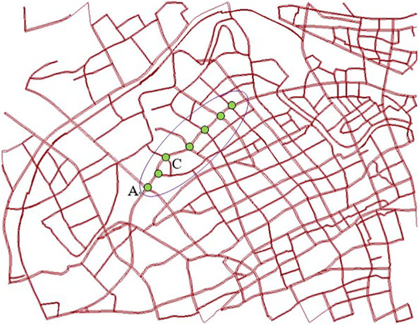
Experimental area schematic.

Figure 5.

Traffic signal phase diagram. (a) Traffic signal phase of intersection A. (b) Traffic signal phase of intersection C.

Intersection A and intersection C are equipped with video detectors. The license plate recognition rate is 99%, and the accuracy rate is 95% (daytime) − 90% (night). The video detector codes of the East and west entrance of the intersection C are 1 and 4, respectively, and the video detector codes of the East and west entrance of the intersection A are 2 and 3, respectively. The schematic diagram of the experimental segment is shown in Figure 6.

Figure 6.

The schematic diagram of the experimental segment.

In this article, the link travel time based on the license plate recognition data of the video detector is taken as the true value. Considering the particularity of the license plate recognition video detector layout, the section between two consecutive intersections is called a road section unit, and the section between two consecutive video detectors is called a combination road section. Due to the travel time, true value of the road section unit cannot be obtained, and the estimation effect of the travel time of the combination road section is only evaluated. The combination road sections A–C and C–A are taken as research objects, and the experimental data are divided into two parts: calibration set and test set. The calibration set accounts for about two-thirds of the total number of data.

The arterial road in the experimental area includes two straight lanes, one left-turn lane, and one straight-right lane. In this article, we only evaluate the travel time estimation effect of the combination road section, so we only take the straight lane as the research object without considering the turning lane. When constructing the feature vector of the traffic pattern, the traffic flow parameter data of the same position coil of the two straight lanes are first averaged. Since the two straight lanes belong to the same phase, the traffic signal control parameter data do not need to be processed similarly.

Parameter calibration

Taking the combination road section A–C as an example, the parameter calibration process of the proposed method is illustrated as follows:

1. Definition of traffic pattern feature vector.

The average traffic data of two straight lane groups at west entrance of intersection B are recorded as ${\bar{q}}_{j, x}$ (B), ${\bar{h}}_{j, x}$ (B), C_j,x(B), g_j,x(B), and DS_j,x(B). The average traffic data of two straight lane groups at west entrance of intersection C are recorded as ${\bar{q}}_{j, x}$ (C), ${\bar{h}}_{j, x}$ (C), C_j,x(C), g_j,x(C), and DS_j,x(C).

2. The selection of the nearest neighbor number K.

Based on the Euclidean distance, the average of the K travel times corresponding to the similar pattern searched is used as the estimated value. The determination of the K value is based on the minimum error of the estimated travel time. When selecting different K values, the mean absolute percent error (MAPE) of the travel time estimation is shown in Figure 7.

Figure 7.

Error measures of travel time estimation under different K.

As can be seen from Figure 7, when K is taken as 4, MAPE is relatively small. Therefore, the nearest neighbor K is selected as 4.

3. Parameter optimization.

In order to determine the best value for C and g, the grid search method is used to optimize the parameters. Meanwhile, the K-fold cross-validation method is used to prevent over-fitting and under-fitting. The training data set is randomly divided into K subset, the LSSVR model is built using K − 1 subset as the training set. The performance of the parameters is checked on the Kth subset. In this article, Gauss RBF is used as kernel function and fivefold cross-validation method is used. Parameter optimization results are shown in Figure 8.

Figure 8.

Parameter optimization results.

As we can see from Figure 8, the optimal parameters of LSSVR model are C = 0.70711, g = 256.

Performance evaluation index

In order to evaluate the efficiency of the proposed approach, three different types of statistical indices are utilized to measure the estimation accuracy. These indices are the mean absolute error (MAE), MAPE, and root mean square error (RMSE). The equations of these indices are as follows

MAE = \frac{1}{n} \sum_{i = 1}^{n} | y_{i} - {\hat{y}}_{i} |

(15)

MAPE = \frac{1}{n} \sum_{i = 1}^{n} | \frac{y_{i} - {\hat{y}}_{i}}{y_{i}} |

(16)

RMSE = \sqrt{\frac{1}{n} \sum_{i = 1}^{n} {| {\hat{y}}_{i} - y_{i} |}^{2}}

(17)

where y_i denotes the actual value for the ith time interval, ${\hat{y}}_{i}$ denotes the estimation value for the ith time interval, n is the total number of time intervals.

Analysis of experimental results

In order to illustrate the estimation performance of the proposed method intuitively, Figure 9 presents estimation results of combination road section A–C.

Figure 9.

Travel time estimation results of combination road section A–C.

As we can see from Figure 9, the travel time estimation result of section A–C has a good trend consistency with its true value. Most of the relative errors are within 10%, and only a few are more than 20%. Most of the absolute error is within 20 s, but the absolute error is large at 17:25:00–18:45:00, which indicates that the travel time estimation effect is not good under severe congestion.

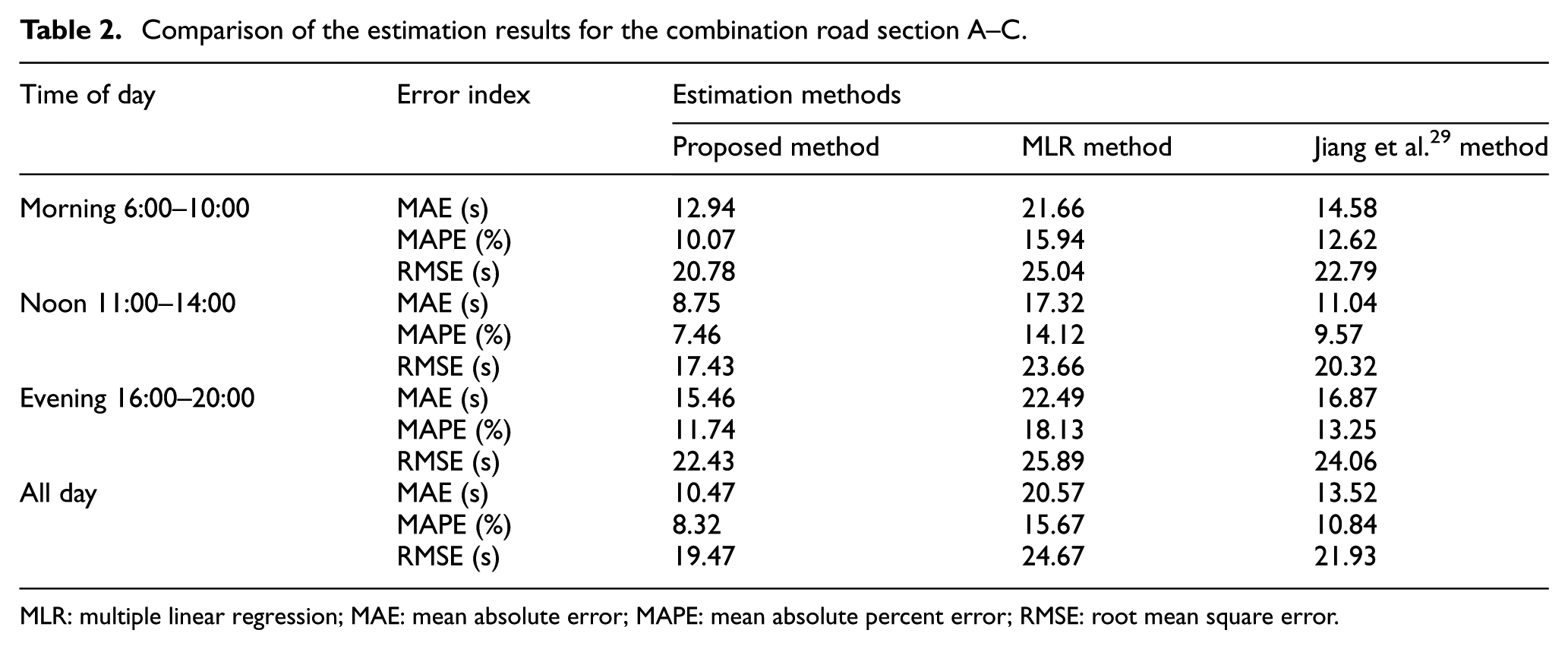
Considering different traffic conditions in different time periods, we selected three periods across the day, including morning peak (6:00–10:00), noon off-peak (11:00–14:00), and evening peak (16:00–20:00) to test performance of the proposed method. In the model validation, we compare the travel time estimation performance of the proposed method with the multiple linear regression (MLR) model and Jiang et al.²⁹ method. Table 2 provides the estimation results of the combination road section A–C. Table 3 provides the estimation results of the combination road section C–A.

Table 2.

Comparison of the estimation results for the combination road section A–C.

Time of day	Error index	Estimation methods
Time of day	Error index	Proposed method	MLR method	Jiang et al.²⁹ method
Morning 6:00–10:00	MAE (s)	12.94	21.66	14.58
	MAPE (%)	10.07	15.94	12.62
	RMSE (s)	20.78	25.04	22.79
Noon 11:00–14:00	MAE (s)	8.75	17.32	11.04
	MAPE (%)	7.46	14.12	9.57
	RMSE (s)	17.43	23.66	20.32
Evening 16:00–20:00	MAE (s)	15.46	22.49	16.87
	MAPE (%)	11.74	18.13	13.25
	RMSE (s)	22.43	25.89	24.06
All day	MAE (s)	10.47	20.57	13.52
	MAPE (%)	8.32	15.67	10.84
	RMSE (s)	19.47	24.67	21.93

MLR: multiple linear regression; MAE: mean absolute error; MAPE: mean absolute percent error; RMSE: root mean square error.

Table 3.

Comparison of the estimation results for the combination road section C–A.

Time of day	Error index	Estimation methods
Time of day	Error index	Proposed method	MLR method	Jiang et al.²⁹ method
Morning 6:00–10:00	MAE (s)	12.97	22.46	14.78
	MAPE (%)	11.05	16.34	13.52
	RMSE (s)	21.94	27.04	23.69
Noon 11:00–14:00	MAE (s)	11.45	19.84	12.94
	MAPE (%)	9.21	15.32	11.35
	RMSE (s)	20.52	25.71	23.57
Evening 16:00–20:00	MAE (s)	16.55	24.59	18.73
	MAPE (%)	12.71	19.16	14.74
	RMSE (s)	24.12	27.79	26.46
All day	MAE (s)	11.59	20.48	13.98
	MAPE (%)	9.35	16.35	11.74
	RMSE (s)	22.68	26.48	24.15

MLR: multiple linear regression; MAE: mean absolute error; MAPE: mean absolute percent error; RMSE: root mean square error.

To consider different patterns of travel time according to the time of day, we compare the travel time estimation results in three periods: morning, noon, and evening. From Tables 2 and 3, we can see that the estimation errors in morning and evening periods were generally higher than those in the noon period. Furthermore, the proposed method is superior to the other two methods both in three periods and all-day. We obtain similar analyzing results for both sections C–A and A-C, which demonstrates that the proposed method has good generalization ability.

Conclusion

Arterial travel time is an important performance measure for both road travelers and traffic engineers. The KNN-LSSVR method is proposed to estimate the arterial travel time based on data commonly provided by SCATS system loop detectors (flow and time headway) and the signal settings (cycle length, green times, and DS value) at each traffic signal. The main contribution of this article is that we propose the concept of a virtual time series to process the original data of the SCATS system and construct a KNN-LSSVR model to estimate arterial travel time. Finally, validation of the travel time estimates has been carried out by using the observed travel times collected from SCATS traffic control system on the arterial road of Shanghai, China. The validation results indicate that the proposed method has a good potential to be developed and is suitable for arterial travel time estimation.

Due to the limitation of the current engineering conditions, this article fails to analyze the travel time estimation effect of the natural section. In addition, the application effect on other roads also needs to be further verified. Further research will be carried out to consider the effects of other factors, such as adverse weather and traffic accidents.

Footnotes

Acknowledgements

The authors express their sincere appreciation to the National Natural Science Foundation of China (no. 51678320).

Handling Editor: Liping Jiang

Declaration of conflicting interests

The author(s) declared no potential conflicts of interest with respect to the research, authorship, and/or publication of this article.

Funding

The author(s) disclosed receipt of the following financial support for the research, authorship, and/or publication of this article: This research was supported by a grant (no. 51678320) from the National Natural Science Foundation of China.

ORCID iD

Qichun Bing

References

Smith

Holt

Park

. Travel time estimation for urban freeway performance measurement: understanding and improving upon the extrapolation method. In: 83rd annual meeting of Transportation Research Board, Washington, DC, 11–15 January 2004, pp.1–20. Washington, DC: National Research Council.

Cavar

Kavran

Bosnjak

Estimation of travel times on signalized arterials. J Civ Eng Archit 2013; 7: 1141–1149.

Tam

Lam

Using automatic vehicle identification data for travel time estimation in Hong Kong. Transp Metr 2008; 4: 179–194.

Chan

Tam

Lam

. Using automatic vehicle identification data for estimating current travel times in Hong Kong. In: 86rd annual meeting of Transportation Research Board, Washington, DC, 21–25 January 2007. Washington, DC: National Research Council.

Zheng

Zuylen

Urban link travel time estimation based on sparse probe vehicle data. Transport Res C 2013; 31: 145–157.

Lin

Long

Real-time estimation of urban street segment travel time using buses as speed probes. Transp Res Rec 2009; 21: 81–89.

Mahmood

Haris

Koutsopoulos Erik

. Travel time estimation from sparse floating car data with consistent path inference: a fixed point approach. Transport Res C 2017: 628–643.

Tang

Chen

Liu

A tensor-based Bayesian probabilistic model for citywide personalized travel time estimation. Transport Res C 2018; 90: 260–280.

Soriguera

Thorson

Robuste

Travel time measurement using toll infrastructure. In: 86rd annual meeting of Transportation Research Board, Washington, DC, 21–25 January 2007. Washington, DC: National Research Council.

10.

Namkoong

Smith

Lee

. A method to estimate path-travel time on expressway using toll collection system data. In: 15th world congress on intelligent transport systems and ITS America’s annual meeting, New York, 16–20 November 2008. Washington, DC: ITS America.

11.

Yoo

Kang

Park

Travel time estimation using mobile data. Proc E Asia Soc Tran 2005; 5: 1533–1547.

12.

Wunnava

Yen

Babji

Travel time estimation using cell phones for highways and roadways. Final report, Florida International University, Miami, FL, January 2007.

13.

Tao

Manolopoulos

Rodriguez

Real-time urban traffic state estimation with A-GPS mobile phones as probes. J Transp Technol 2012; 2: 22–31.

14.

Cherrett

Bell

McDonald

Estimatingvehicle speed using single inductive loop detectors. P I Civil Eng: Transp 2001; 147: 23–32.

15.

Vanajakshi

Williams

Rilett

Improvedflow-based travel time estimation method from point detector data for freeways. J Transp Eng 2009; 135: 26–36.

16.

Skabardonis

Geroliminis

. Real-time estimation of travel times on signalized arterials. In: Proceedings of the 16th international symposium on transportation and traffic theory, College Park, MD, 19–21 July 2005, pp.387–406.

17.

Liu

Real-time estimation of arterial travel time under congested conditions. Transportmetrica 2012; 8: 87–104.

18.

Rose

Sarvi

Evaluation of speed-based travel time estimation models. J Transp Eng 2006; 132: 540–547.

19.

Van Lint

JWC

van der Zijpp

. Improving a travel-time estimation algorithm by using dual loop detectors. J Transp Res Rec 2003; 1855: 41–48.

20.

Bhaskar

Chung

Dumont

AG.

Analysis for the use of cumulative plots for travel time estimation on signalized network. Int J Intell Transp Syst Res 2010; 8: 151–163.

21.

Kwon

Coifman

Bickel

Day to day travel time trends and travel time prediction from loop detector data. Transp Res Rec 2000; 1717: 120–129.

22.

Robinson

Polak

Modeling urban link travel time with inductive loop detector data by using the k-NN method. Transp Res Rec 2005; 1935: 47–56.

23.

Tang

Zou

Ash

et al . Travel time estimation using freeway point detector data based on evolving fuzzy neural inference system. PLoS ONE 2016; 11: e0147263.

24.

Liu

van Lint

JWC

van Zuylen

. Neural network based traffic flow model for urban arterial travel time prediction. In: 86rd annual meeting of Transportation Research Board, Washington, DC, 21–25 January 2007. Washington, DC: National Research Council.

25.

Zhu

Guo

Polak

et al . Urban link travel time estimation using traffic states-based data fusion. IET Intell Transp Syst 2018; 12: 651–663.

26.

Luk

Karl

et al . Real-time estimation of travel times on arterial roads in Melbourne. In: 22nd ARRB conference: research into practice, Canberra, ACT, Australia, 29 October–2 November 2006. Vermont South, VIC, Australia: ARRB Group Ltd.

27.

Mazloumi

Currie

Rose

Using SCATS data to predict bus travel time. In: 32nd Australasian transport research forum (ATRF), Auckland, 29 September–1 October 2009.

28.

Cheu

Liu

Lee

Arterial travel time estimation using SCATS detectors. In: Proceedings of the 7th international applications of advanced technologies in transportation engineering, Canbridge, MA, 5–7 August 2002. Cambridge: American Society of Civil Engineers.

29.

Jiang

Dong

Travel time estimation method using SCATS traffic data based on K-NN algorithm. J Southwest Jiaotong Univ 2013; 48: 343–349.

30.

Mack

YP.

Local properties of k-NN regression estimates. J Algebraic Discr Meth 1981; 2: 311–323.

Arterial travel time estimation method using SCATS traffic data based on KNN-LSSVR model

Abstract

Keywords

Introduction

Feature analysis and processing of SCATS data

Characteristics analysis of SCATS traffic data

Construction of virtual time series for SCATS traffic data

Arterial travel time estimation based on KNN-LSSVM model

KNN search mechanism

The principle of LSSVR model

Modeling of travel time estimation based on KNN-LSSVR

Empirical analysis

Design of experimental scheme

Parameter calibration

Performance evaluation index

Analysis of experimental results

Conclusion

Footnotes

Acknowledgements

Declaration of conflicting interests

Funding

ORCID iD

References