Sage Journals: Discover world-class research

Abstract

Diagnostic health monitoring without prior knowledge is still a hard problem in the prognostic and health management field. A multivariate diagnostic health monitoring strategy is proposed based on telemetry data for in-orbit spacecrafts with component degradation. Compared with the existing univariate or direct diagnostic health monitoring methods, multivariate diagnostic health monitoring methods can avoid constructing one-dimensional synthesized health index and setting empirical thresholds for different health states. In our developed strategy, a deep forest algorithm combined with an effective feature extraction approach and fuzzy C-means clustering algorithm is proposed to achieve more accurate assessment of the current health state. First, a partitioning window is utilized to deal with the raw telemetry data and then features which have high monotonicity and trends are extracted for diagnostic health monitoring. Then, a fuzzy C-means algorithm is used to handle unlabeled telemetry data and determine states of degrading component. Finally, a deep forest classifier is adopted to obtain the prognostic model for online probabilistic diagnostic health monitoring. Verification results on a simulated spacecraft attitude control system can demonstrate the effectiveness and feasibility of the proposed multivariate diagnostic health monitoring strategy.

Keywords

Diagnostic health monitoring feature extraction deep forest spacecraft attitude control system

Introduction

Prognostic and health management (PHM) technology is important to various spacecrafts for successful task management, orbital maintenance, and service life prolongation. PHM technologically focuses on predicting the health status of a system by assessing the deviation from the expected normal operating condition. The deviation is usually caused by faults, failures, or component degradations.¹ Specifically, PHM can be used for two purposes:² diagnostic health monitoring and prognostic health monitoring. Diagnostic health monitoring is to evaluate the current health status of a component, subsystem, or system, whereas prognostic health monitoring is to predict the future trends of the degradation process and the remaining useful life. This article focuses on developing a novel and effective strategy for diagnostic health monitoring of in-orbit spacecrafts.

The existing diagnostic health monitoring approaches are generally classified into three major categories: physical model-based approaches,^3–5 data-driven approaches,^6–8 and hybrid approaches.^9–11 Physical model-based approaches require the physical understanding of the object and can be successfully applied to material-level or component-level objects. However, these techniques are rarely used for macro levels, such as systems or subsystems. Because obtaining system-level models for diagnostic health monitoring with affordable efforts is difficult or even impossible in many large-scale applications. Data-driven approaches fulfill diagnostic health monitoring using data mining, pattern recognition, and machine learning techniques to the accessible life cycle data of the object. Hybrid approaches are developed based on available multi-source information, including physical model, operating data, or expert knowledge. For in-orbit spacecrafts, many telemetry data containing rich information on the health states are available. Therefore, data-driven approaches are usually utilized for the diagnostic health monitoring of spacecrafts.

Data-driven approaches for diagnostic health monitoring can be further categorized into the following groups: univariate health index–based approaches,¹² direct approaches,¹³ and multivariate approaches.¹⁴ Univariate approaches need to establish a one-dimensional (1D) synthesized health index (SHI) using linear regression,¹⁵ principal component analysis (PCA),^2,16 and Mahalanobis distance.^17,18 The thresholds for identifying different health states of the devices or systems during their life cycles must be predefined. However, constructing effective SHIs and defining accurate thresholds are difficult because of time-varying operating condition, environment, noisy measurements, and high-level uncertainties in real applications. The direct approaches achieve diagnostic health monitoring by matching the current observation trajectories with the most similar historical trajectories. However, complete run-to-failure data are rare, and similarity searching¹⁹ can be time-consuming, for systems with numerous variables. Multivariate approaches^7,20,21 are newly emerging techniques that automatically divide the health degradation process into several stages using unsupervised clustering algorithms and then label the current health state by searching the nearest cluster. Compared with the former two approaches, the multivariate approaches do not need to establish a 1D SHI, predefine the thresholds of different health states, or have a large number of similar historical samples. However, the existing multivariate approaches rarely consider the uncertainties of different health states and health state switching process. Moreover, many unsolved problems still exist in real applications.²⁰

For in-orbit spacecrafts, the health-relevant telemetry data often have the following features:

1. Multi-dimensional degradation signals.

We take attitude control system (ACS) as an example. The ACS contains controller, flywheel, and other components. Therefore, the collected telemetry data from ACS is multi-dimensional. In addition, one component degradation signal can influence other components due to the failure propagation of closed-loop structure. These component signals having degradation features are called multi-dimensional degradation signals.

2. Multi-domain degradation features.

The degradation feature of one component signal may not be evident due to noise masking and closed-loop compensation. Therefore, the raw signal should be excavated in multiple domains (time, frequency, and time–frequency domains). These excavated features of one component signal may directly reflect the degradation phenomenon. This is called multi-domain degradation features.

3. Huge unlabeled and unbalanced data.

No indicator can directly represent the health states or transitions between different health states due to the lack of available prior knowledge. This is called unlabeled problem. In addition, the telemetry data are not well balanced temporally or spatially, which is called unbalanced problem in the field of machine learning. For example, abundant data can be found for health or subhealth status during their life cycles, whereas the data close to the failure stage of degradation is extremely rare.

4. High-level uncertainties.

Spacecrafts’ health monitoring is affected by various sources and high-level uncertainties. Spacecrafts have different in-orbit tasks, which usually change orbit altitude and condition environment. This kind of uncertainty is induced by environmental and operational conditions. Furthermore, ground station observation limit, closed-loop compensation, and different initial stages are also the sources of different uncertainties. In addition, the difficulty of constructing SHIs and the dynamics of health thresholds also cause these uncertainties.

A feasible and effective data-driven diagnostic health monitoring strategy for in-orbit spacecrafts is needed to solve the following basic problems:

How to extract multi-domain health-degradation-relevant features from massive multivariate telemetry data?

How to deal with huge unlabeled and unbalanced telemetry data of spacecrafts?

How to deal with the uncertainties in telemetry data?

In order to solve the shortcomings of the existing multivariate approaches and real application restricts, a feasible and effective multivariate diagnostic health monitoring strategy for in-orbit spacecrafts based on deep forest is proposed in this article. First, a multi-domain feature extraction and evaluation method is proposed to automatically extract health-degradation-relevant features. A fuzzy C-means clustering (FCM) algorithm is then utilized to deal with the huge unlabeled and unbalanced telemetry data of spacecrafts by dynamically dividing the health states into four stages. Finally, a deep forest classifier is adopted for the probabilistic assessment of health states, and the probabilistic results can represent the uncertainties of health state switching process.

The remainder of this article is organized as follows. Section “Multi-domain degradation feature extraction and evaluation” presents a multi-domain degradation feature extraction method. Then, a multivariate diagnostic health monitoring approach is proposed in section “Multivariate diagnostic health monitoring based on deep forest classifier,” using a deep forest classifier combined with an FCM algorithm. Verification results are shown in section “Verification,” by a simulation platform of satellite ACS with gyroscope degradation. Finally, conclusions are drawn in section “Conclusion.”

Multi-domain degradation feature extraction and evaluation

Degradation feature extraction and evaluation are the foundation of diagnostic health monitoring. In general, the features with high monotonicity and trends can reflect the degradation of a system’s health performance. In this section, multi-domain features are extracted from the telemetry data. Given that the multi-domain features of each variable can be highly redundant, feature evaluation is necessary to select the most representative features and guarantee the efficiency of the proposed method. In this article, a strategy (Figure 1) is proposed. This strategy contains telemetry data preprocessing (data compression), multi-domain feature extraction, and feature evaluation (smoothing, feature selection, cumulative sum, and normalization).

Figure 1.

The strategy of multi-domain degradation feature extraction and evaluation.

Telemetry data preprocessing

The available telemetry data can be arranged into three-dimensional (3D) data $X (I \times J \times K_{I})$ (Figure 2), where I represents the number of spacecraft samples, and i is the index of the spacecraft sample $(i = 1, \dots, I)$ ; J represents the number of monitoring variables, and j is the index of the monitoring variable $(j = 1, \dots, J)$ ; $K_{I}$ represents the operational cycle of spacecraft samples, and k is the index of the operational cycle $(k = 1, \dots, K_{I})$ . A spacecraft sample contains the whole life cycle data in one simulation.

Figure 2.

The schematic of telemetry data.

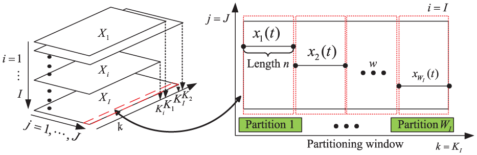
When $i = I$ , $j = J$ , and $k = K_{I}$ , the data become a two-dimensional (2D) time series (Figure 3). The right image in Figure 3 is the enlarged drawing of the left red region, and a partitioning window is used for data compression. In data compression, $x_{w} (t)$ represents the time series of partition w; $t = 1, 2, \dots, n$ and n is the length of each partitioning window; $w = 1, 2, 3, \dots, W_{I}$ and $W_{I}$ is the total number of partitioning windows. In general, n is selected as 1 min, 1 h, or 1 day divided by the sampling period. In this article, 1 day is the standard.

Figure 3.

Partitioning window for data compression.

Multi-domain feature extraction

Time-domain features

In this section, each time series $x_{w} (t)$ is used to calculate different features, from $1$ to $W_{I}$ . Time-domain feature extraction^22,23 is based on the common statistical characteristic parameters as shown in Table 1. These features are generally divided into two groups: dimensional and non-dimensional time-domain features. The first 11 features are dimensional time-domain features, and the rest are non-dimensional time-domain features. In the dimensional time-domain features, the mean usually reflects the change of wear; the root mean square usually reflects the vibration amplitude and energy of a signal; the variance usually reflects the fluctuate of a signal; the standard deviation usually measures the amount of variance from mean; the peak and peak-to-peak usually reflect the influence degree of a signal. In the non-dimensional time-domain features, the influence of the work environment is usually eliminated. In total, time-domain features are sensitive to the change in amplitude or distribution and are suitable to provide global information on the health state.

Table 1.

Time-domain statistical characteristic parameters.

Index	Feature	Calculation formula
1	Mean	$M = \frac{1}{n} \sum_{t = 1}^{n} x_{w} (t)$
2	Absolute mean	$AM = \frac{1}{n} \sum_{t = 1}^{n} \| x_{w} (t) \|$
3	Root mean square	$RMS = \sqrt{\frac{1}{n} \sum_{t = 1}^{n} x_{w}^{2} (t)}$
4	Average power	$AVP = \frac{1}{n} \sum_{t = 1}^{n} x_{w}^{2} (t)$
5	Root amplitude	$ROA = {(\frac{1}{n} \sum_{t = 1}^{n} \sqrt{\| x_{w} (t) \|})}^{2}$
6	Peak	$PE = max (\| x_{w} (t) \|)$
7	Peak-to-peak	$PEP = max (x_{w} (t)) - min (x_{w} (t))$
8	Variance	$VA = \frac{1}{n - 1} \sum_{t = 1}^{n} (x_{w} (t) - M)^{2}$
9	Standard deviation	$STD = \sqrt{\frac{1}{n - 1} \sum_{t = 1}^{n} {(x_{w} (t) - M)}^{2}}$
10	Skewness	$SK = \frac{1}{n} \sum_{t = 1}^{n} (x_{w} (t) - M)^{3}$
11	Kurtosis	$KU = \frac{1}{n} \sum_{t = 1}^{n} (x_{w} (t) - M)^{4}$
12	Waveform index	$WAI = RMS / AM$
13	Crest index	$CRI = PE / RMS$
14	Impulse index	$IMI = PE / AM$
15	Margin index	$MAI = PE / ROA$
16	Skewness index	$SKI = SK / ST D^{3}$
17	Kurtosis index	$KUI = KU / ST D^{4}$

Frequency-domain features

In-orbit spacecraft’s telemetry data often exhibit complicated periodicity due to its orbital period, the observation period, and the rhythm of day and night. The health degradation process may be influenced by certain periodical features, so frequency-domain features should be extracted to reveal some useful information uncovered in the time-domain features. In this article, five typical frequency-domain features^22,23 are listed in Table 2. Frequency center, mean square frequency, and root mean square frequency show the position changes of the main frequencies. Root mean square frequency, variance frequency, and root variance frequency describe the convergence degree of the spectrum power.

Table 2.

Frequency-domain statistical characteristic parameters.

Index	Feature	Calculation formula
1	Frequency center	$\underset{=}{FC} \sum_{t = 2}^{n} x_{w} (t) {\overset{\cdot}{x}}_{w} (t) / 2 π \sum_{t = 1}^{n} x_{w}^{2} (t)$
2	Mean square frequency	$MSF = \sum_{t = 2}^{n} {\overset{\cdot}{x}}_{w}^{2} (t) / 4 π^{2} \sum_{t = 1}^{n} x_{w}^{2} (t)$
3	Root mean square frequency	$RMSF = \sqrt{MSF}$
4	Variance frequency	$VF = MSF - (FC)^{2}$
5	Root variance frequency	$RVF = \sqrt{VF}$

${\overset{\cdot}{x}}_{w} (t) = (x_{w} (t) - x_{w} (t - 1)) / Δ$ , and $Δ$ is the sample interval.

Time–frequency-domain features

For non-stationary and non-periodic signals, time–frequency-domain analysis is more suitable than time-domain or frequency-domain analysis. The most common approaches of time–frequency-domain analysis are empirical mode decomposition (EMD), wavelet transform (WT), and wavelet packet transform (WPT). EMD is time-consuming and is not suitable for plenty of telemetry data. Compared with WT, WPT is a precise signal analysis method. Therefore, the WPT is adopted, and a four-level wavelet packet decomposition^22,24 is employed according to engineering experience in this article. The length of partitioning window is enough for the four-level wavelet packet decomposition. Figure 4 shows the fourth-level WPT decomposition of the time series signal $x_{w} (t)$ . In this article, the energy entropy $H_{x_{w}}$ is extracted as the time–frequency-domain feature. Mathematically, the feature can be calculated as the following

\begin{matrix} x_{w} (t) = \sum_{o = 1}^{2^{d}} x_{w, d}^{o} (t) \end{matrix}

(1)

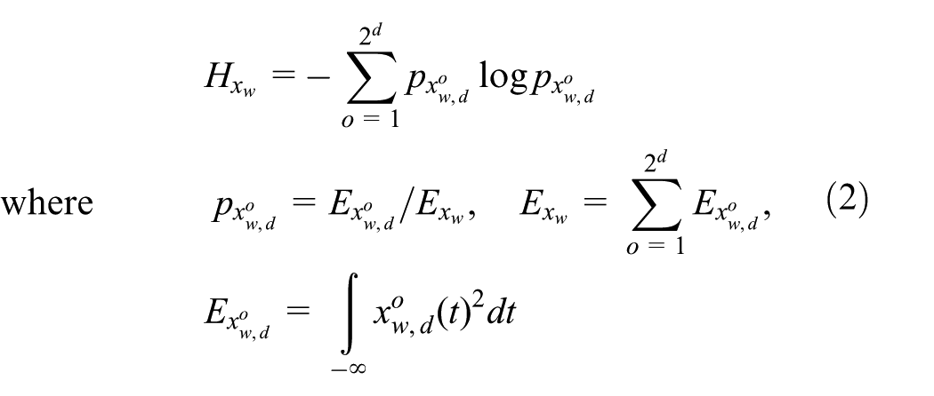
where integers $o (o = 1, 2, \dots, 2^{d})$ and $d (d = 4)$ are the modulation and the scale, respectively; $x_{w, d}^{o} (t)$ is the wavelet packet component signal

\begin{matrix} H_{x_{w}} = - \sum_{o = 1}^{2^{d}} p_{x_{w, d}^{o}} \log p_{x_{w, d}^{o}} \\ where p_{x_{w, d}^{o}} = E_{x_{w, d}^{o}} / E_{x_{w}}, E_{x_{w}} = \sum_{o = 1}^{2^{d}} E_{x_{w, d}^{o}}, \\ E_{x_{w, d}^{o}} = \int_{- \infty} x_{w, d}^{o} {(t)}^{2} dt \end{matrix}

(2)

where $p_{x_{w, d}^{o}}$ is the percentage of energy $E_{x_{w, d}^{o}}$ of oth wavelet packet component signal in the whole signal energy $E_{x_{w}}$ .

Figure 4.

Diagram of four-level wavelet packet transform.

Feature evaluation

This section aims to eliminate the redundant features and maintain the most representative features to guarantee the efficiency of the online diagnostic health monitoring. Therefore, the main steps contain data smoothing, correlation calculation, feature selection, cumulative sum, and normalization.

First, feature smoothing²⁵ is suitable for feature selection and cumulative sum. The local regression using weighted linear least squares and a first-degree polynomial model²⁶ is then adopted. This method has the simplicity of the traditional linear regression and the flexibility of nonlinear regression.

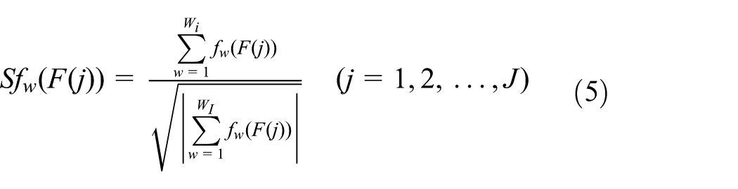
Second, Spearman correlation coefficient method²⁷ is employed for feature selection. Spearman correlation analysis is an unsupervised feature selection method that does not have specific data condition, as compared with two other correlation analysis methods (Pearson and Kendall). Figure 5 shows the correlation calculation process of multi-domain features. Twenty-three multi-domain features $f_{w} (l)$ are calculated in each time series $x_{w} (t)$ , and l is the index of features $(l = 1, 2, \dots, 23)$ . For the variable J, $f_{1} (l), f_{2} (l), \dots, f_{w} (l)$ comprise the $l th$ feature time series in each sample i. The time series correlation coefficient $ρ_{l, i} (J)$ is calculated according to equation (3)

ρ_{l, i} (J) = 1 - \frac{6 \sum_{w = 1}^{W_{i}} d_{f_{w} (l)}^{2}}{{W_{i}}^{3} - W_{i}}

(3)

where $d_{f_{w} (l)}^{2}$ represents the difference between ranks for the $l th$ feature time series in each sample i and this time series operational time.

Figure 5.

Correlation calculation process of multi-domain features.

Other time series correlation coefficients are calculated similarly as above, and 23 correlation coefficients $ρ_{1, i} (J), ρ_{2, i} (J), \dots, ρ_{23, i} (J)$ are also calculated in each sample i. The above is the calculative process for the variable J correlation coefficients and for other variables.

The feature selection for variable J can be considered as a multi-objective optimization problem that contains two constraint conditions. One is that each correlation coefficient absolute value of feature l in sample i must be greater than threshold $θ$ . The other is that correlation coefficients of feature l in all samples are greater than 0 or less than 0. If feature l meets the above conditions, then the sum of feature l in all samples must be calculated. For the variable J, the index corresponding to the maximal sum absolute value is the final result $F (J)$ . For each variable, no more than one optimal feature (among the 23 extracted features) can be selected. The specific formula can be summarized as follows, and feature selections of other variables are the same

\begin{matrix} \begin{matrix} F (J) = \underset{l}{\arg} max {| \sum_{i = 1}^{I} ρ_{l, i} (J) | / I (l = 1, 2, \dots, 23)} \\ s . t . | ρ_{l, i} (J) | \geq θ (i = 1, 2, \dots, I) \\ no . of ρ_{l, i} (J) > 0 = I or \\ no . of ρ_{l, i} (J) < 0 = I \end{matrix} \end{matrix}

(4)

where $F (J)$ is the optimal feature index of the variable J; $θ$ is a threshold of feature selection and is set to 0.5 in this article; $no .$ represents the number of the features with the increasing or decreasing trends.

Third, the extracted features are calculated using a cumulative sum function.²⁵ The sum function furnishes a running total for a given time series $f_{w} (F (j))$ in each sample i as below. The results of the cumulative sum can be considered as the new 3D feature data sets $Y (I \times W_{I} \times J)$

\begin{matrix} S f_{w} (F (j)) = \frac{\sum_{w = 1}^{W_{i}} f_{w} (F (j))}{\sqrt{| \sum_{w = 1}^{W_{I}} f_{w} (F (j)) |}} (j = 1, 2, \dots, J) \end{matrix}

(5)

where $S f_{w} (F (j))$ represents the selected feature cumulative sum of variable j up to the end in sample i.

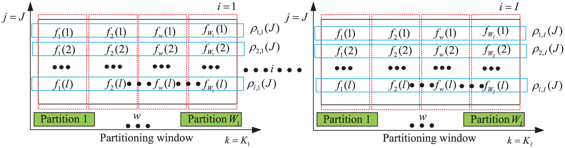
Finally, to solve the uncertainties caused by different initial stages and lengths of data sets, we reshape the 3D data $Y (I \times W_{I} \times J)$ into the 2D data sets $Y (Z \times J) (Z = W_{1} + W_{2} + \dots + W_{I})$ according to variable J²⁸ as shown in Figure 6. This normalization method does not consider whether the data length of each sample is consistent. Equation (6) gives the specific calculation process. The mean ${\bar{y}}_{j}$ and variance $s_{j}$ are also suitable for the online data normalization of multivariate diagnostic health monitoring

\begin{matrix} {\tilde{y}}_{zj} = \frac{y_{zj} - {\bar{y}}_{j}}{s_{j}} \\ where {\bar{y}}_{j} = \frac{1}{Z} \sum_{z = 1}^{Z} y_{zj} \\ s_{j} = \sqrt{\frac{1}{Z - 1} \sum_{z = 1}^{Z} {(y_{zj} - {\bar{y}}_{j})}^{2}} \end{matrix}

(6)

Figure 6.

Normalization of three-dimensional data.

Multivariate diagnostic health monitoring based on deep forest classifier

Key idea

In multivariate health monitoring, the deep forest classifier²⁹ combined with FCM is adopted to assess the current health state, as shown in Figure 7. This method can be divided into two phases. Phase I provides the FCM algorithm for health state classification and avoids directly defining the empirical thresholds of different health states. Four health states (normal, slight damage, medium damage, and failure) are defined in this article. Phase II utilizes the deep forest classifier for offline training and online health state assessment.

Figure 7.

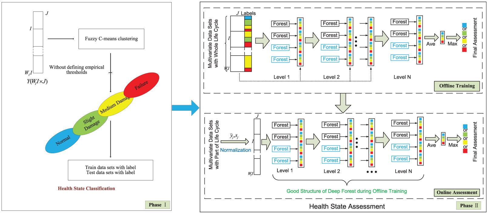
The scheme of multivariate diagnostic health monitoring based on deep forest.

Health state classification

Defining the different health states of degradation process is necessary to enhance the precision of multivariate diagnostic health monitoring modeling without expert knowledge. Moreover, dealing with the uncertainty of transitions among different health states is also important.

Therefore, we apply the FCM algorithm to solve this uncertainty due to fuzzy sets. FCM³⁰ is a clustering method that allows one piece of data to belong to two or more clusters. FCM is frequently used in pattern recognition. This clustering algorithm can also divide the expanded 2D-normalized data sets of degradation into four dynamic discrete health stages: normal, slight damage, medium damage, and failure, rather than static ones based on fixed values³¹ and the assumed continuous observations.^31–33 The method is suitable for degrading machinery, and the detailed descriptions of FCM are given below.

Given the 2D data sets $Y (Z \times J)$ , FCM is based on minimization of the following objective function

\begin{matrix} L = \sum_{c = 1}^{C} \sum_{z = 1}^{Z} {[μ_{c} (y_{z})]}^{b} | | y_{z} - m_{c} {| |}^{2}, 1 < b < \infty \end{matrix}

(7)

where b is set to 2; $Y (Z \times J) = {y_{1}, y_{2}, \dots, y_{z}, \dots, y_{Z}}^{T}$ and $y_{z} = {y_{z 1}, y_{z 2}, \dots, y_{zJ}}^{T}$ ; $μ_{c} (y_{wi})$ is the degree of membership of $y_{wi}$ in the cluster c; and $m_{c} (c = 1, 2, \dots, C)$ is the center of the cluster.

Fuzzy partitioning is applied through an iterative optimization of the objective function as shown above, with the update of the cluster centers $m_{c}$ and membership $μ_{c} (y_{z})$ by

\begin{matrix} m_{c} = \frac{\sum_{z = 1}^{Z} {[μ_{c} (y_{z})]}^{b} y_{z}}{\sum_{z = 1}^{Z} {[μ_{c} (y_{z})]}^{b}} \end{matrix}

(8)

\begin{matrix} μ_{c} (y_{z}) = \frac{| | y_{z} - m_{c} {| |}^{- 2 / (b - 1)}}{\sum_{c = 1}^{C} | | y_{z} - m_{c} {| |}^{- 2 / (b - 1)}} \end{matrix}

(9)

This iteration stops when $max_{cz} {| μ_{c} (y_{z})^{k + 1} - μ_{c} (y_{z})^{k} |} < ε$ , where $ε$ is a termination criterion between 0 and 1, whereas k is the number of iteration step. This procedure converges to a local minimum or a saddle point of L. FCM is composed of the following steps:

Step 1: initialize $U = [μ_{c} (y_{z})]$ matrix, $U^{(0)}$ .

Step 2: at k-step, calculate the centers vectors $M^{(k)} = [m_{c}]$ with $U^{(k)}$ using equation (8).

Step 3: update $U^{(k)}$ and $U^{(k + 1)}$ using equation (9).

Step 4: if $U^{(k + 1)} - U^{(k)} < ε$ , then stop; otherwise, return to Step 2.

Diagnostic health monitoring

In Figure 7, the diagnostic health monitoring is divided into offline training and online assessment. In the offline training, data sets with whole life cycles are trained to acquire and save the good structure of deep forest. In the online assessment, data sets with part of life cycles are first normalized using ${\bar{y}}_{j}$ , and $s_{j}$ are then applied to online health state assessment using the saved good structure of deep forest. The deep forest is suitable for the rare data that are close to the failure stage of degradation. To our knowledge, this work is the first to apply the deep forest algorithm to diagnostic health monitoring.

The deep forest classifier is inspired by the layer-by-layer structure of deep neural network. This algorithm employs a forest cascade structure, including two complete-random forests (black)³⁴ and two random forests (blue)³⁵ in each level as shown in Figure 7. Each complete-random forest or random forest contains huge complete-random decision trees or random decision trees. The number of trees in each forest is a hyper-parameter, and the value will be given later. Each complete-random tree is generated by randomly selecting a feature in each tree node. The tree then grows until each node contains the same instance or has no more than 10 instances. Similarly, each random decision tree is generated by selecting the optimal Gini value in $\sqrt{q}$ candidate features (q is the number of input features). For the given sample set V, the Gini can be obtained by equation (10)

\begin{matrix} Gini (V) = 1 - \sum_{g = 1}^{G} {(\frac{V_{g}}{V})}^{2} \end{matrix}

(10)

where $V_{g}$ is the sample subset which belongs to the class g and G is the number of class.

If the given sample set V is divided into $V_{1}$ and $V_{2}$ by one possible value a of feature, then the Gini will be defined by equation (11)

\begin{matrix} Gini (V, A) = \frac{| V_{1} |}{| V |} Gini (V_{1}) + \frac{| V_{2} |}{| V |} Gini (V_{2}) \end{matrix}

(11)

The $Gini (V, A)$ presents the uncertainty of the sample set V by splitting through $A = a$ ; Similar to entropy, the value of $Gini (V, A)$ presents the uncertainty degree. Hence, the optimal Gini index is selected as $a^{*} = \underset{a \in A}{\arg} min Gini (V, A = a)$ .

Each level cascade receives a feature vector generated by its previous level and outputs the processed feature vector to the next level. This cascade structure can usually guarantee to achieve a global solution.

Figure 8 gives the brief algorithm flow of deep forest classifier. The algorithm flow mainly contains multi-gained scanning, first-layer forest, and forest concatenate. In multi-gained scanning, the training data sets, and labels entered are divided into training samples and validation samples. Then, the algorithm uses sliding windows to cut time series sets, similar to convolutional neural network (CNN). In the first-layer forest, the time series sets are used to train random and complete-random forests. The out-of-bag estimation is then calculated. In forest concatenate, a new level is extended, and the accuracy of the cascade layer is evaluated. The assessment probabilities of this cascade layer are then provided, and the performance improvement is evaluated. If the performance is not obvious evident, then the assessment results are outputted. Otherwise, the forest concatenate is continued.

Figure 8.

Algorithm flow of deep forest.

The deep forest can give a probabilistic assessment result. First, we introduce how each forest can generate possibilities of different classes as illustrated in Figure 9. In a forest, the input is the preceding-level feature vector and each tree can estimate the percentage of different classes at its leaf node. The forest can then generate the whole class distribution by averaging the above estimations of all trees. The generated class vector of different forests in the level is the input feature vector of the next level. When the performance improvement is not evident (similar to the above), the averaging class vectors of all forests in the last level become the final different class distributions. Finally, the maximum of different class distributions is the probabilistic assessment result. In this article, the parameters of the deep forest algorithm are shown as follows

\begin{matrix} \begin{matrix} n_cascadeRF = 2 \\ n_cascadeRFtree = 101 \\ cascade_test_size = 0.2 \\ tolance = 0 \end{matrix} \end{matrix}

where n_cascadeRF is the number of complete-random forests or random forests in a cascade layer; n_cascadeRFtree is the number of trees in a single random forest in a cascade layer; cascade_test_size is the split fraction for cascade training set splitting; and tolance is the accuracy tolerance for the cascade growth.

Figure 9.

Probabilistic results of deep forest.

In conclusion, the implementation details of the deep forest based diagnostic health monitoring can be summarized in Algorithm 1.

Algorithm 1. Multivariate diagnostic health monitoring
Input: -Training data sets and test data sets
- The accuracy flag $N_accuracy$
Output: -The current health state
Process:
1: Utilize training data sets with whole life cycle and labels to train deep forest.
2: for $i = 1, 2, \dots, n$ do
3: Calculate prediction accuracy $accuracy_i$ of the sample i.
4: if $accuracy_i \geq 90 %$ then
5: $N_accuracy = N_accuracy + 1$
6: end if
7: end for
8: if $N_accuracy = = n$ then
9: Save the structure of deep forest.
10: else
11: Repeat the above Steps.
12: end if
13: Normalize test data sets using ${\bar{y}}_{j}$ and $s_{j}$ .
14: Import the structure to assess the current health state.

Verification

ACS simulation platform

In this section, we utilize the ACS simulation platform to simulate and produce telemetry data. The minisatellite team (belongs to College of Astronautics, Nanjing University of Aeronautics and Astronautics) used stochastic hybrid automata (SHA) method to exploit the platform in MATLAB Simulink environment. This platform can simulate environmental disturbance, fault injection, and component degradation. Several control algorithms and fault diagnosis methods are studied and verified theoretically based on this platform before TX-1 minisatellite is sent into space.

This platform contains seven modules: PD control; four-inclined reaction wheel; triaxial magnetorquer; satellite kinematics and dynamics; triaxial star sensor; fiber optic gyroscope subsystem; and environment disturbance and orbit as shown in Figure 10. The symbol description of this platform is listed in Table 3. We use the platform to simulate the gradual degradation of gyroscope subsystem (Figure 11). The gyroscope subsystem is a hot-backup structure and has two gyroscopes in each axis. In each simulation, we stop the simulation and record the telemetry data when two gyroscopes in any axis have broken down. The variables of indexes 4, 8, 13, and 14 are 13 simulated telemetry data. The sample period is 10 s.

Figure 10.

Diagram of simulation platform.

Table 3.

Symbol description of ACS simulation platform.

Index	Symbol	Physical meanings	Unit
1	$[ϕ_{E}, θ_{E}, ψ_{E}]$	Expected values of attitude angle	°
2	$[Δ ϕ, Δ θ, Δ ψ]$	Errors of attitude angle	°
3	$[\overset{\cdot}{\hat{ϕ}}, \overset{\cdot}{\hat{θ}}, \overset{\cdot}{\hat{ψ}}]$	Measured values of attitude angle velocity	°/s
4	$[n_{1}, n_{2}, n_{3}, n_{4}]$	Actual speeds of reaction wheel	r/min
5	$M_{W}$	Moments of control command	$A m^{2}$
6	${\hat{M}}_{W}$	Actual moments of reaction wheel	$A m^{2}$
7	$M_{M}$	Moments of uninstall command	$A m^{2}$
8	${\hat{M}}_{M}$	Actual moments of magnetorquer	$A m^{2}$
9	$ω_{0}$	Angular velocity of orbit	°/s
10	$M_{E}$	Disturbance moments	$A m^{2}$
11	$[ϕ, θ, ψ]$	Actual attitude angle	°
12	$[ω_{x}, ω_{y}, ω_{z}]$	Actual values of body axis rotation	°/s
13	$[\hat{ϕ}, \hat{θ}, \hat{ψ}]$	Measured values of attitude angle	°
14	$[{\hat{ω}}_{x}, {\hat{ω}}_{y}, {\hat{ω}}_{z}]$	Measured angular velocity of star	°/s

ACS: attitude control system.

Figure 11.

Configuration of gyrosystem.

In this article, nine samples $(9 \times 13 \times K_{I})$ are produced by the simulation platform to verify the effectiveness of the proposed strategy. Five samples with whole life cycle and two samples with whole life cycle are randomly selected for offline training and testing, respectively. The rest of the samples with parts of life cycle are selected for online health state assessment.

Data processing

Each sample produced by the above platform is 3–5 GB, which severely affects the processing speed of health diagnostic health monitoring algorithm. Therefore, features that can define degradation must be extracted for data processing.

In this section, we explain the process of feature extraction and evaluation in detail by taking the variable $n_{1}$ as an example. The variable $n_{1}$ represents the actual rotational speed of the first reaction wheel during the spacecraft operation. Figure 12 gives the raw data of $n_{1}$ , and the number of raw data is as high as $3 \times 10^{7}$ . Furthermore, the raw data do not exhibit evident degradation. Hence, directly utilizing the raw data for diagnostic health monitoring is difficult and time-consuming.

Figure 12.

Raw data of $n_{1}$ .

First, the partitioning window technology is adopted for data compression. The window length is set to 8460 $(8640 \times 10 s = 1 day)$ and then the 23 multi-domain features of $n_{1}$ are calculated in each partitioning window. Limited by paper space, only three main time-domain features of $n_{1}$ are shown in Figure 13. Frequency-domain features and time–frequency-domain features of $n_{1}$ are, respectively, shown in Figures 14 and 15(a). Compared with the time coordinate of Figures 12 –15(a), data compression by partitioning window is achieved successfully, and data number decreases obviously from $3 \times 10^{7}$ to $3 \times 10^{3}$ . The frequency-domain and time–frequency-domain features exhibit degradation compared with time-domain features. However, $n_{1}$ has many unnecessary features and one optimal feature must be selected.

Figure 13.

Several time-domain features of $n_{1}$ .

Figure 14.

Frequency-domain features of $n_{1}$ .

Figure 15.

Feature extraction of $n_{1}$ : (a) selected feature and (b) cumulative result of selected feature.

Second, according to equations (3) and (4), the value of $F (n_{1})$ is 13. Therefore, the wavelet packet energy entropy of $n_{1}$ is the optimal feature. Similar to the optimal feature selection of $n_{1}$ , the optimal features of 12 other variables are listed in Table 4.

Table 4.

Optimal features of telemetry variables.

Telemetry variable	Optimal feature
$[\hat{ϕ}, \hat{θ}, \hat{ψ}]$	Mean
${\hat{ω}}_{x}$	Mean
${\hat{ω}}_{y}$	Peak
${\hat{ω}}_{z}$	Peak-to-peak
$[n_{1}, n_{2}, n_{3}, n_{4}]$	Wavelet packet energy entropy
${\hat{M}}_{M}$	Wavelet packet energy entropy

Finally, the cumulative sum of the wavelet packet energy entropy is calculated by equation (5), and the result is shown in Figure 15(b). For the variable $n_{1}$ , the cumulative sum result of wavelet packet energy entropy is a good monitoring index for health state assessment.

Diagnostic health monitoring

In the offline training, the whole extracted features of different samples are first normalized by equation (6) uniformly, and the mean and variance of this normalized are saved. Second, FCM is utilized to label different health states as shown in Figure 16. The labels of health states are injected by FCM to deal with the unlabeled and unbalanced data. In Figure 16, “1” represents normal state, “2” represents slight damage state, “3” represents medium damage state, and “4” represents failure state. In the two top images of Figure 16, the black solid line represents the labeled health states (actual states) by FCM. The red imaginary line presents the training result using the deep forest classifier. In the two bottom images of Figure 16, the blue solid line represents the health probability of corresponding top data in the same time. From Figure 16, the accuracy rates of offline training are all above 95%, and only several misclassifications are found in the transitions among different health states. In addition, the probabilistic results of transitions among different health states are low and can accurately reflect the uncertainty of transitions among different health states. Finally, the good structure of forest in offline training is saved for online health state assessment.

Figure 16.

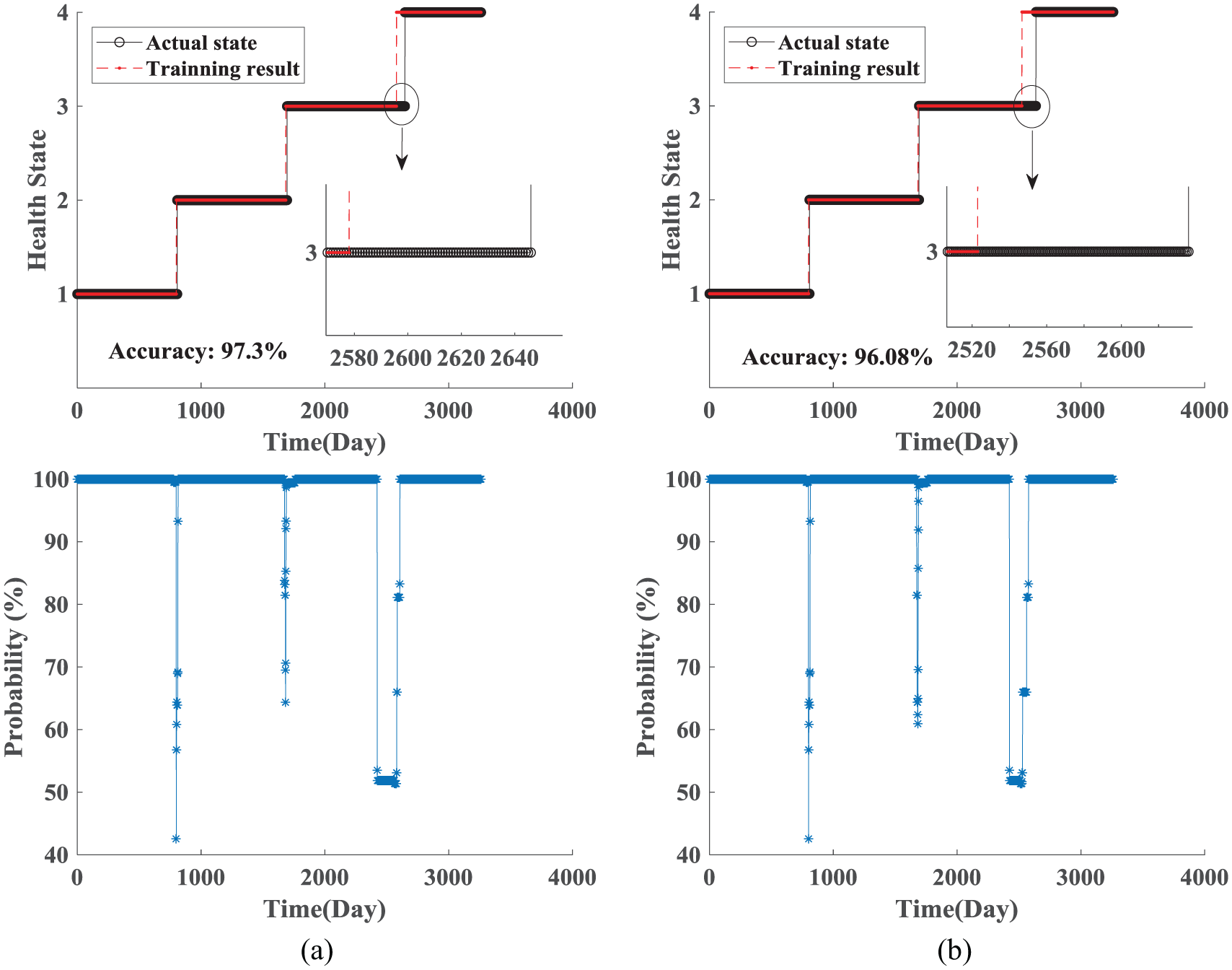
Offline training: (a) sample 1 and (b) sample 2.

In the online health state assessment, we first utilize the saved mean and variance to normalize the rest samples, which are parts of life cycle from the normal stage to the end of the third stage. Second, the well-trained structure of forest in offline training is adopted to assess the current health state of the rest samples. Finally, the results of online health state assessment are shown in Figure 17. From Figure 17, the accuracy rates of online prediction are all above 90%, and few misclassifications are found between the transition points before 2500 days. In addition, the health states are assessed as failure state in advance, and the corresponding probabilistic results are lower than 75%. In fact, the low probability indicates that the system is not in a real failure state. The change of health state will be accepted only when the probabilistic value becomes 90%. These results show the benefits of the proposed method.

Figure 17.

Online health state assessment.

According to all these results, either offline training or online prediction shows that the probabilistic multivariate diagnostic health monitoring is better than general methods. Deep forest classifier can be successfully applied for health state assessment.

Conclusion

The multivariate diagnostic health monitoring, combined with effective feature extraction, FCM, and deep forest classifier, has been proposed to solve the problem of SHI construction and empirical thresholds setting in the PHM field. This method can extract multi-domain health-degradation-relevant features from a given mass of multivariate telemetry data, and can deal with unlabeled and unbalanced spacecraft telemetry data and the uncertainties in these data. The offline training and online health state assessment results on the simulated ACS of a spacecraft reveal the feasibility and effectiveness of the proposed strategy.

However, prognostic health monitoring is as important as diagnostic health monitoring in the PHM field. Its main purpose is to predict the trend of the next degradation stages and even the remaining useful life. In the future, the prognostic health monitoring will be considered.

Footnotes

Handling Editor: Nuno Maia

Declaration of conflicting interests

The author(s) declared no potential conflicts of interest with respect to the research, authorship, and/or publication of this article.

Funding

The author(s) disclosed receipt of the following financial support for the research, authorship, and/or publication of this article: This work was supported by the Nature Science Foundation of China under grants 61873122 and 61673206, Equipment Pre-research National Defense Science Technology Key Laboratory Foundation under grant 61422080307, Key Laboratory of Spacecraft Fault Diagnosis and Maintenance on Orbit, and Postgraduate Research & Practice Innovation Program of Jiangsu Province under grant KYCX18_0300.

ORCID iDs

Ningyun Lu

Yuehua Cheng

References

Pecht

Prognostics and health management of electronics. Hoboken, NJ: John Wiley & Sons, 2009, pp.222–229.

Moghaddass

Zuo

MJ.

An integrated framework for online diagnostic and prognostic health monitoring using a multistate deterioration process. Reliabil Eng System Safet 2014; 124: 92–104.

Bressel

Hilairet

Hissel

et al . Extended Kalman filter for prognostic of proton exchange membrane fuel cell. Appl Ener 2016; 164: 220–227.

Tagade

Hariharan

Gambhire

et al . Recursive Bayesian filtering framework for lithium-ion cell state estimation. J Power Sources 2016; 306: 274–288.

Chi

KRL

Mba

. Switching Kalman filter for failure prognostic. Mech Syst Signal Process 2015; 52–53: 426–435.

Tobon-Mejia

Medjaher

Zerhouni

CNC machine tool’s wear diagnostic and prognostic by using dynamic Bayesian networks. Mech Syst Signal Process 2012; 28: 167–182.

Zhou

Huang

Reduced kernel recursive least squares algorithm for aero-engine degradation prediction. Mech Syst Signal Process 2017; 95: 446–467.

Wang

Jiang

et al . Dynamic fault prognosis for multivariate degradation process. Neurocomputing 2018; 275: 1112–1120.

Pennacchi

Chatterton

Vania

et al . Experimental evidences in bearing diagnostics for traction system of high speed trains. Chem Eng Trans 2013; 33: 739–744.

10.

Hong

Wang

et al . In situ health monitoring for bogie systems of CRH380 train on Beijing–Shanghai high-speed railway. Mech Syst Signal Process 2014; 45: 378–395.

11.

Pillai

Kaushik

Bhavikatti

et al . A hybrid approach for fusing physics and data for failure prediction. Int J Prognost Health Manage 2016; 7: 1–12.

12.

Wang

Youn

A generic probabilistic framework for structural health prognostics and uncertainty management. Mech Syst Signal Process 2012; 28: 622–637.

13.

Ramasso

Rombaut

Zerhouni

Prognostic by classification of predictions combining similarity-based estimation and belief functions. In: Denoeux

Masson

(eds) Belief functions: theory and applications. New York: Springer, 2012, pp.61–68.

14.

Javed

Gouriveau

Zerhouni

. Novel failure prognostics approach with dynamic thresholds for machine degradation. In: IECON 2013-39th annual conference of the IEEE industrial electronics society, Vienna, 10–13 November 2013, pp.4404–4409. New York: IEEE.

15.

Wang

Siegel

et al . A similarity-based prognostics approach for remaining useful life estimation of engineered systems. In: 2008 prognostics and health management conference, Denver, CO, 6–9 October 2008, pp.1–6.

16.

A nonlinear probabilistic method and contribution analysis for machine condition monitoring. Mech Syst Signal Process 2013; 37: 293–314.

17.

Tamilselvan

Wang

Failure diagnosis using deep belief learning based health state classification. Reliabil Eng Syst Safety 2013; 115: 124–135.

18.

Lin

Chen

Zhou

Online probabilistic operational safety assessment of multi-mode engineering systems using Bayesian methods. Reliabil Eng Syst Safety 2013; 119: 150–157.

19.

You

Meng

A framework of similarity-based residual life prediction approaches using degradation histories with failure, preventive maintenance, and suspension events. Electr Prod Reliabil Environ Testing 2012; 62: 127–135.

20.

Javed

Gouriveau

Zerhouni

A new multivariate approach for prognostics based on extreme learning machine and fuzzy clustering. IEEE Trans Cybernet 2015; 45: 2626–2639.

21.

Gouriveau

Medjaher

Zerhouni

From prognostics and health systems management to predictive maintenance 1: monitoring and prognostics. Hoboken, NJ: John Wiley & Sons, 2016, pp.88–97.

22.

Lei

Zuo

et al . A multidimensional hybrid intelligent method for gear fault diagnosis. Expert Syst Applicat 2010; 37: 1419–1430.

23.

Ilya

Kirill

Panagiotis

Machine learning search for variable stars. Monthly Notices Royal Astron Soc 2018; 475: 2326–2343.

24.

Sun

Chang

CC.

Structural damage assessment based on wavelet packet transform. J Struct Eng 2002; 128: 1354–1361.

25.

Javed

Gouriveau

Zerhouni

et al . A feature extraction procedure based on trigonometric functions and cumulative descriptors to enhance prognostics modeling. In: 2013 prognostics and health management conference, Gaithersburg, MD, 24–27 June 2013, pp.1–7. New York: IEEE.

26.

Moran

Lewis

PAW

. Locally-weighted-regression scatter-plot smoothing (LOWESS): a graphical exploratory data analysis technique thesis advisor. Thesis Collection, 1984, https://apps.dtic.mil/dtic/tr/fulltext/u2/a152239.pdf

27.

Gautheir

TD.

Detecting trends using spearman’s rank correlation coefficient. Environ Foren 2001; 2: 359–362.

28.

Louwerse

Smilde

AK.

Multivariate statistical process control of batch processes based on three-way models. Chem Eng Sci 2000; 55: 1225–1235.

29.

Zhou

Feng

Deep forest: towards an alternative to deep neural networks. arXiv, 2017, https://arxiv.org/abs/1702.08835

30.

Dunn

JC.

A fuzzy relative of the isodata process and its use in detecting compact well-separated clusters. J Cybernet 1974; 3: 32–57.

31.

Ramasso

Rombaut

Zerhouni

Joint prediction of continuous and discrete states in time-series based on belief functions. IEEE Trans Syst Man Cybernet 2012; 43: 37–50.

32.

Ramasso

Gouriveau

. Prognostics in switching systems: evidential Markovian classification of real-time neuro-fuzzy predictions. In: 2010 prognostics and health management conference, Macao, China, 12–14 January 2010, pp.1–10. New York: IEEE.

33.

Javed

Gouriveau

Zemouri

et al . Features selection procedure for prognostics: an approach based on predictability. In: 8th IFAC international symposium on fault detection, supervision and safety for technical processes, Mexico City, Mexico, 29–31 August 2012, pp.25–30. New York: IEEE.

34.

Fan

Wang

et al . Is random model better? On its accuracy and efficiency. In: 3rd IEEE international conference on data mining, Melbourne, FL, 22 November 2003, pp.51–58. New York: IEEE.

35.

Breiman

Random forest. Machine Learning 2001; 45: 5–32.

A telemetry data based diagnostic health monitoring strategy for in-orbit spacecrafts with component degradation

Abstract

Keywords

Introduction

Multi-domain degradation feature extraction and evaluation

Telemetry data preprocessing

Multi-domain feature extraction

Time-domain features

Frequency-domain features

Time–frequency-domain features

Feature evaluation

Multivariate diagnostic health monitoring based on deep forest classifier

Key idea

Health state classification

Diagnostic health monitoring

Verification

ACS simulation platform

Data processing

Diagnostic health monitoring

Conclusion

Footnotes

Declaration of conflicting interests

Funding

ORCID iDs

References