
Abstract
With the development of theory and advancement of scientific research, fractional calculus has begun to be considered as a method for the study of physical systems. In this work, based on the basic system of equations for internal solitary waves, we have derived two-dimensional Benjamin–Ono equation. Then, the integer-order two-dimensional Benjamin–Ono equation is transformed into the time-fractional Benjamin–Ono equation. To study the properties of the algebraic internal solitary waves, we discuss the conservation laws of the new model. Also, using the Hirota bilinear method, the derived new model is solved. Finally, we explore the characteristics of motion of the algebraic internal solitary waves with the help of the multi-soliton solutions.
Keywords
Introduction
Nonlinear partial differential equations have been used to describe a wide range of physics phenomena as a model for the evolution and interaction of nonlinear waves.1–8 Particularly, internal solitary waves are a commonly occuring feature along the belt of the continental edge with suitable stratification, current, and topography. The research on the internal waves is a research hot spot and various applications have been found in ocean engineering, global environment, and underwater acoustic exploration.9–15 Algebraic solitary wave theory is an important part of the study of nonlinear partial differential equation. This type of equation admits exact solutions representing “algebraic” solitary waves.16–18 In recent years, the application of fractional differential equations has attracted increasing attention in many different areas.19–26 Researchers have discovered that the derivatives and integrals of fractional order models are suitable for describing various physical phenomena.
Conservation laws are a mathematical formulation which indicates that the total amount of a certain physical quantity remains the same during the evolution of a physical system. Conservation laws provide much information as regards systems simulated by differential equations. 27 Many fractional conservation laws were obtained in the past two decades.26–32
Many solution methods have been found and used to solve the fractional order equation, for instance, the homotopy perturbation method, 33 Hirota bilinear method,34,35 computational approach, 36 and others.37–44 Various phenomena can be explained via the application of the solutions given by the above methods.45–47 Approximation and numerical methods such as variational iteration and adomian decomposition have been used because most fractional differential equations do not have exact analytic solutions. In recent years, Odibat and Momani have realized the solution method of fractional order nonlinear ordinary differential equation. They use the homotopy perturbation method to derive analytic approximate solution of the nonlinear partial differential equation of a fractional order system.
Since the concept of soliton was first put forward, the solution of integral partial differential development equation has been one of the most important research topics.48–51 For fractional partial differential equations, how to obtain the soliton solutions of a nonlinear wave equation is also of great research value. Recently, the Hirota bilinear method has been used to solve fractional models. This method is one direct and efficient way for obtaining the multi-solitary wave solutions. In this article, we obtain soliton solutions for the new model using the Hirota bilinear method.
This article is organized as follows. Section “Derivation of the 2D BO equation” is devoted to the derivation of the two-dimensional (2D) Benjamin–Ono (BO) equation which can describe the internal wave propagation in a deep stratified fluid. In section “Formulation of the time-fractional BO equation,” the resultant BO equation is converted into the time-fractional BO equation. In section “Conservation laws of the time-fractional BO equation,” conservation laws of the time-fractional BO equation are discussed. In section “Multi-soliton solutions for the time-fractional BO equation,” we seek multiple-soliton solutions of the equation using the simplified Hirota bilinear method. And then, based on the analytic solutions of the BO equation, the propagation of the two-solitary waves are discussed and illustrated. Section “Conclusion” contains the results and discussion of this work.
Derivation of the 2D BO equation
We shall begin by considering an inviscid, incompressible, density-stratified fluid with boundary conditions of infinite depth. Initially, we shall suppose that the flow is three dimensional (3D) and can be described by the spatial coordinates
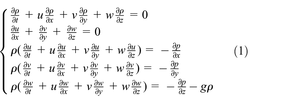
where t is the time variable, g is the gravitational acceleration, u, v, and w are the three fluid velocity components in the x-, y-, and z-directions, respectively,
The boundary conditions are

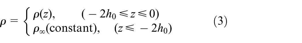
and the density is defined as
Now we consider the flow in the upper layer

where

The variables are expanded in the following form

where
Substituting equations (5) and (6) into equation (1), we can obtain the approximate equations for

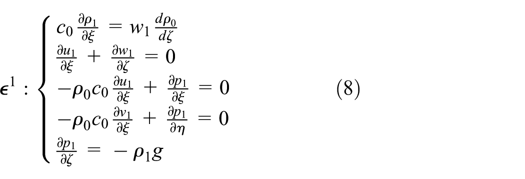

where
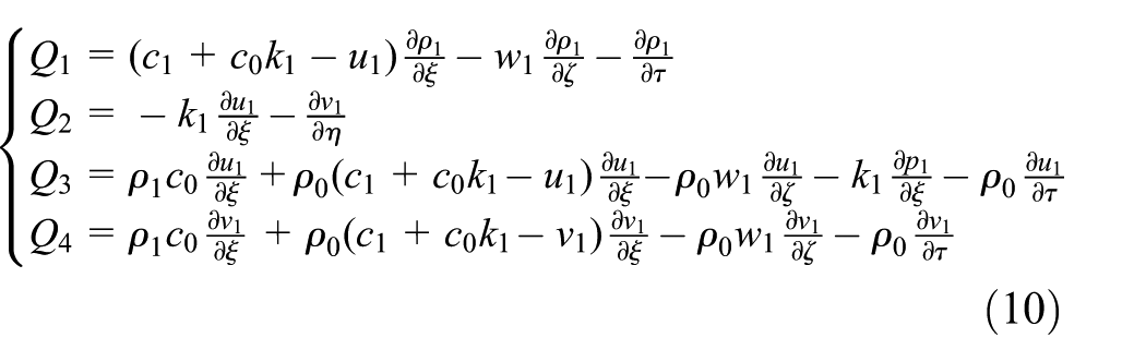
Eliminating
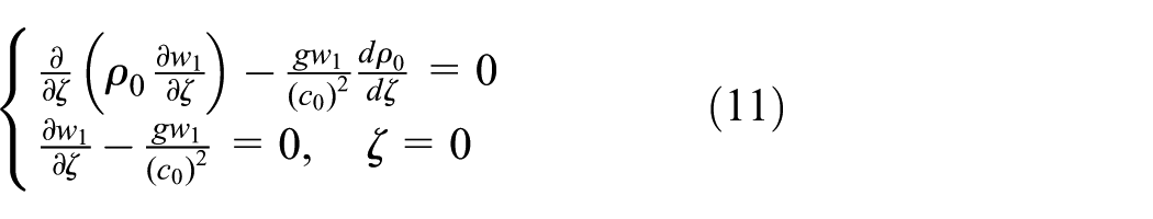
To solve the above equations, we suppose that the solution to equation (11) is written as follows
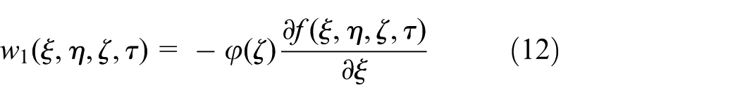
where f denotes the wave amplitude which acquires

Substituting equations (12) and (13) into equation (11), we can obtain the governing equation and the boundary condition of

Also, by equation (12), we can rewrite
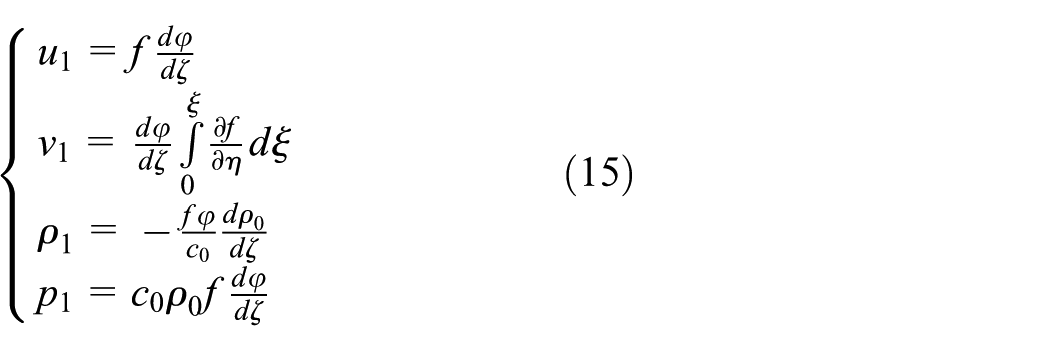
Eliminating
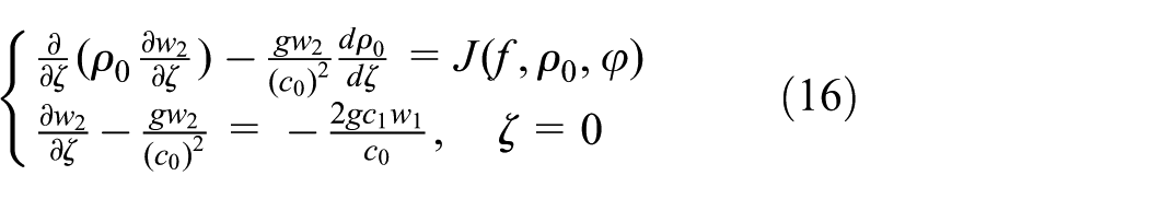
where

By equation (15), we can rewrite
where

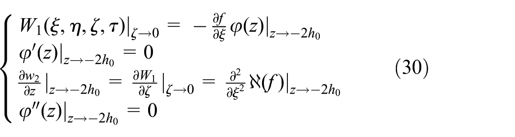
By the solvable condition of
we obtain

where

Next, we consider the flow in the lower layer

and thus we can obtain

The variables are expanded in the following form

Substituting equations (24) and (25) into equation (1), we can obtain the following equation

and the boundary condition of

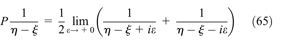
The solution to equation (26) with boundary conditions is the principal value of Cauchy integral

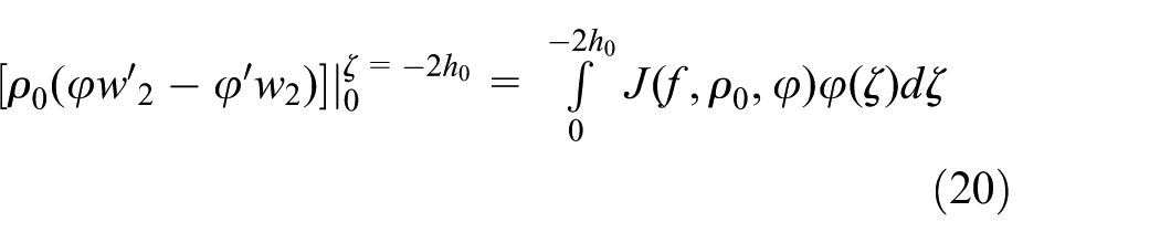
Taking the derivative with respect to

Matching the value of the lower layer and the upper layer at
where

is the famous Hilbert transformation. Then setting

Now setting

which is the 2D BO equation.
Formulation of the time-fractional BO equation
In section “Derivation of the 2D BO equation,” we have obtained the 2D BO equation. In this section, the BO equation will be converted to the time-fractional BO equation.
According to the BO equation (33), assuming

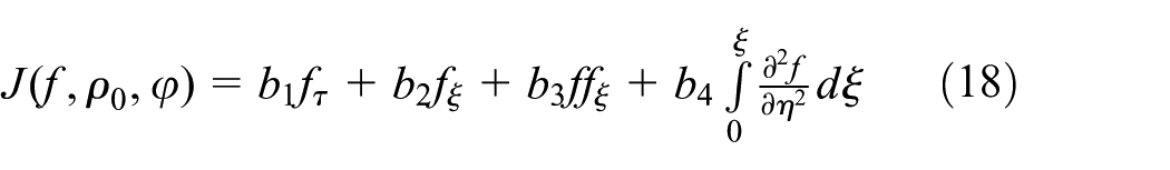
Then, the functional of the potential equation (34) can be described as
where

Using the variation of the above function, we obtain

Comparing equation (34) with equation (37), we obtain the following Lagrangian multipliers

Therefore, the Lagrangian form of the BO equation is given by

Similarly, the Lagrangian form of the time-fractional BO equation is given by

where the fractional derivative

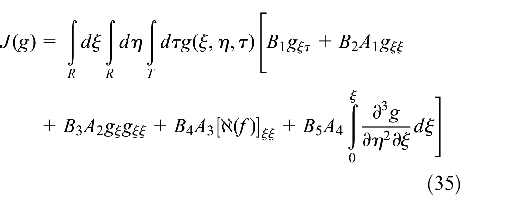
Thus, the functional of the time-fractional BO equation can be obtained as

According to Agrawal’s method, the variation of the functional (equation (42)) can be written as

The fractional integration by parts satisfies the following rules

and

Using the fractional integration by parts for equation (43), we can obtain

Optimizing the variation (equation (46)) and setting

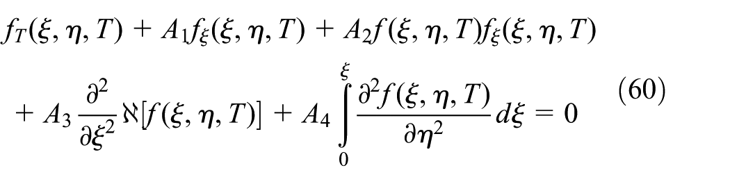
Substituting equation (40) into equation (47), we have

Substituting

which is the time-fractional BO equation.
Conservation laws of the time-fractional BO equation
In this section, we will discuss conservation laws of the time-fractional BO equation to learn about the properties of the new model (49). First, we assume

Integrating equation (49) with respect to

where
Next, we multiply equation (49) by

and the properties of the Hilbert operator
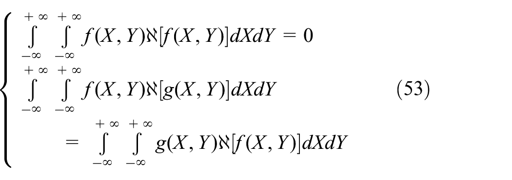
where

where
Now, multiplying equation (49) by

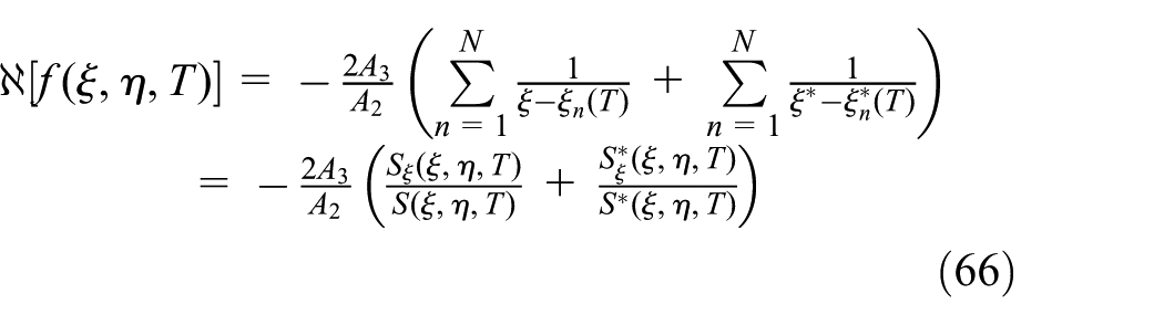
Deriving equation (49) about

Deriving equation (49) about

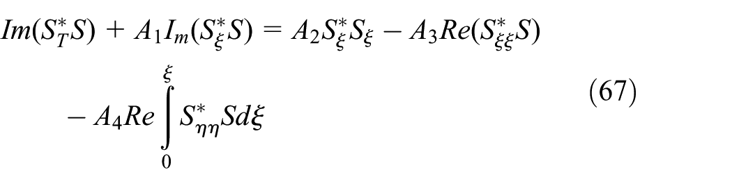
According to the above equations, we obain
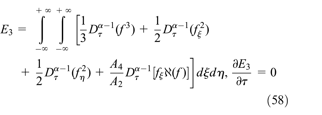
where
Multi-soliton solutions for the time-fractional BO equation
In this section, using the simplified Hirota bilinear method, we seek multiple-soliton solutions of equation (49) and the propagation of the two-solitary waves based on the obtained analytic results.
First, we introduce the following fractional transforms

where p is a constant. Using the above transformations, we can convert equation (49) into
We assume that the solution of equation (60) has the form

where

where
Substituting equation (61) into equation (60), we can obtain
Hence, equation (61) can be written as

Then using formula
we have
Substituting equations (62), (64), and (66) into equation (60), the internal wave BO equation can be transformed to the bilinear form
Based on the bilinear equation (67) and using the bilinear method, the N-solitary wave solution is given in the matrix form
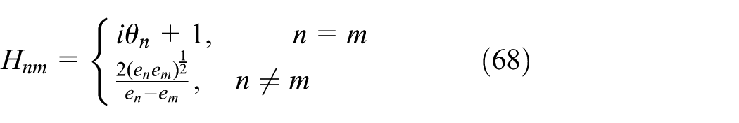
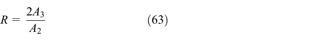
with

where
When

Substituting equation (70) into equation (64), we obtain the one-solitary wave solution

When

where

Substituting equation (72) into equation (64), we obtain the two-solitary wave solution

Now, we rewrite equation (74) as
where

Based on the above conclusion, we can give the images of the two-soliton solution with different fractional orders
As we can see from Figure 1, when

Plots for the two-soliton solution with different fractional orders
In addition to single- and double-soliton wave solutions, there may be three-soliton wave solutions to the equation,52–54 but for the fractional order equation in this article, we only study the first two solutions, and whether and how the three-soliton solutions exist will be the focus of our future research.
Conclusion
In this work, using multi-scale analysis and the perturbation method, we have obtained the 2D BO equation based on the basic system of equations. Furthermore, based on the integer-order model and using the semi-inverse method and the fractional variational principle, we obtain the 2D fractional BO equation which opens the door to the study of internal solitary waves. Also, we study the conservation laws of the new model using the Riemann–Liouville fractional derivative. Then, using the Hirota bilinear method, we obtain the soliton solutions of the new fractional model. Based on the multi-soliton solutions, we study the characteristics of motion of internal solitary waves.
Footnotes
Handling Editor: Dean Vučinić
Declaration of conflicting interests
The author(s) declared no potential conflicts of interest with respect to the research, authorship, and/or publication of this article.
Funding
The author(s) disclosed receipt of the following financial support for the research, authorship, and/or publication of this article: This project was supported by the Nature Science Foundation of Shandong Province of China (Nos ZR2018MA017 and ZR2017BEE033), Open Fund of the Key Laboratory of Meteorological Disaster of Ministry of Education (Nanjing University of Information Science and Technology) (No. KLME201801), National Natural Science Foundation of China (No. 51804180), and Key Research Plan of Shandong Province (No. 2018GSF116007).