Online prediction and control method for compensation regulation value in grinding processes

Abstract

In any grinding process, compensation regulation value is a crucial factor for maintaining precision during the batch processing of workpieces. Geometric characteristics, buffing allowance, temperature, wheel speed, and workpiece speed are the main factors that affect compensation regulation value in any grinding process. In this article, a novel prediction method for compensation regulation value is proposed based on incremental support vector machine and mixed kernel function. The support vectors for the prediction model are extracted using the convex hull vertex optimization algorithm, and the speed of the operation can be increased effectively. In addition, the parameters of the model are optimized using cross-validation optimization method to improve the accuracy of the prediction model. Then, the feedback control strategy of compensation regulation value for the grinding process is also proposed. Single-factor and multi-factor experiments are implemented respectively using the proposed method. The results verify the feasibility and effectiveness of the proposed method. It is also noted that the machining accuracy is improved significantly in comparison with the machining without prediction and compensation control. Moreover, by applying the prediction compensation control of compensation regulation value to the active measurement and control of the grinding process, a feedback system is formed, and then the intelligentization of the grinding system can be realized.

Introduction

Grinding is an important machining method, and the quality of the workpiece is determined by the precision of the grinding process. ¹ In recent years, due to the development of industrial intelligence and automation, the demands for real-time measurement devices and process control instruments for the grinding process are increasing tremendously.^2,3 The cylindrical grinding process can be divided into rough grinding, fine grinding, and buffing (spark-out stage). ⁴ During the grinding process, the grinding wheel moves rapidly into the rough grinding stage. At signal point 2, it enters the fine grinding stage, and at signal point 3, it enters the buffing stage. When the grinding wheel reaches signal point 4, the workpiece returns to the preset size. At different stages, the grinding system parameters (grinding wheel speed, workpiece speed, feed speed, and grinding feed) are different. The sketch map of the grinding process is illustrated in Figure 1.

Figure 1.

Sketch map of grinding process.

In any grinding process, temperature drift causes a deviation in the control system. It is important to adjust the zero loci before the active measurement controller works, thus resulting in a deviation in the dynamic measurement of the workpiece. At the buffing stage, the buffing allowance, wheel speed, and workpiece speed also lead to a deviation. For this kind of deviation, operators use a pneumatic micrometer to measure the deviation and then adjust the signal points of the grinding control system and manually input the compensation values.^5,6 This method of compensation lags behind the grinding process, and hence, the randomness is large. The compensation methods for workpieces of different sizes are not the same and mainly depend on the experience of the operator.

In this article, the online prediction and compensation control function of an active measurement controller in a grinding control system is studied. By judging whether the predicted values of the compensation values exceed the compensation range or not, the machining accuracy and the degree of automation of the grinding process are determined. Through the analysis of various forecasting theories, the error-corrected least-squares support vector machine (LSSVM) is selected as the basis of forecasting theory.^7,8 The prediction and compensation feedback control diagram of compensation regulation value (CRV) is depicted in Figure 2.

Figure 2.

Prediction and compensation feedback control diagram of CRV.

Support vector machine and parameter optimization

LSSVM

The LSSVM, an extension of the support vector machine (SVM), is developed by Suykens. ⁹ The traditional SVM solves the problem of function estimation through quadratic programming,^10,11 whereas LSSVM solves the linear equation problems using the least-squares method to reduce the complexity of the model as well as to improve the speed of the solution.^12,13 During forecasting, the dimension of model data lies from low to high and also from nonlinear to linear. ¹⁴

Let us consider a set of samples $\{({\mathit{x}}_1,y_1),({\mathit{x}}_2,y_2),\dots ,({\mathit{x}}_s,y_s)\}$ , where ${\mathit{x}}_i$ is an n-dimensional input vector, $y_i$ is the output value, and s is the number of samples. The decision function in high-dimensional space can be constructed as

$$f(\mathit{x})={\mathit{w}}^{\mathrm{T}}\phi (\mathit{x})+b$$

(1)

where w is the weight coefficient, $\phi (x)$ is the mapping function, and b is the bias constant.

The formula of structural risk is given by

$$R=\frac{1}{2}c{R}_{\mathrm{emp}}+\frac{1}{2}{\mathit{w}}^{\mathrm{T}}\mathit{w}$$

(2)

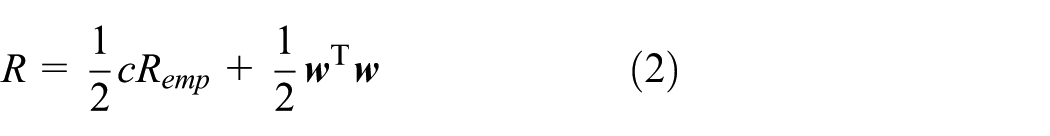
where c is the error penalty factor, $R_{\mathrm{emp}}$ is the loss function ( $R_{\mathrm{emp}}=\sum {{\xi }_i}^2$ ), and ${\xi }_i$ is the slack variable.

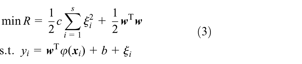
The solution of model parameters is equivalent to the following optimization problem

$$\begin{array}{c}\multicolumn{1}{c}{minR=\frac{1}{2}c\sum _{i=1}^s{\xi }_i^2+\frac{1}{2}{\mathit{w}}^{\mathrm{T}}\mathit{w}}\\ \multicolumn{1}{c}{\mathrm{s}.\mathrm{t}.y_i={\mathit{w}}^{\mathrm{T}}\phi ({\mathit{x}}_i)+b+{\xi }_i}\end{array}$$

(3)

Introducing the Lagrange function based on the Karush–Kuhn–Tucker (KKT) conditions, the solution of the optimization problem can be obtained

$$\begin{array}{c}\multicolumn{1}{c}{L(\mathit{w},b,\xi ,\mathbf{\alpha })=\frac{1}{2}\mathbf{c}\sum _{\mathbf{i}=1}^{\mathbf{s}}{\mathbf{\xi }}_{\mathbf{i}}^2+\frac{1}{2}{\mathit{w}}^{\mathrm{T}}\mathit{w}}\\ \multicolumn{1}{c}{-\sum _{\mathbf{i}=1}^{\mathbf{s}}{\mathbf{\alpha }}_{\mathbf{i}}({\mathit{w}}^{\mathrm{T}}\mathbf{\phi }({\mathit{x}}_{\mathbf{i}})+\mathbf{b}+{\mathbf{\xi }}_{\mathbf{i}}-{\mathbf{y}}_{\mathbf{i}})}\end{array}$$

(4)

where $\mathbf{\alpha }=({\mathbf{\alpha }}_1,{\mathbf{\alpha }}_2,\dots ,{\mathbf{\alpha }}_{\mathbf{s}}{)}^{\mathrm{T}}$ is the Lagrange multiplier. Consequently, a regression model of LSSVM can be achieved

$$f(x)=\sum _{i=1}^s{\alpha }_{i}K({\mathit{x}}_i,{\mathit{x}}_j)+b$$

(5)

where $K(x_i,x_j)$ is the kernel function (i, j = 1, …, s).

In a complex prediction problem, the training data is subordinate to both polynomial distribution and Gaussian distribution. If only the Gaussian kernel function is chosen, the data that obey the polynomial kernel distribution cannot be accurately divided; therefore, the choice of only one class of kernel function could lead to poor prediction. In this article, the mixed kernel function is selected to combine the advantages of single kernel function.^15–17

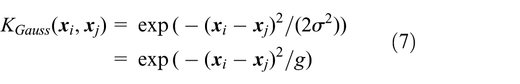
Polynomial kernel function can effectively characterize the global nature of data. The distant points can affect the values of kernel function to make the generalization ability strong; however, the weak learning ability is the main disadvantage. The Gaussian kernel function is the representative of the local kernel function. The points with short distances have profound effects on the values of the kernel function, thus the learning ability is strong, while the generalization ability is weak. When the parameter g tends to zero, the sample may be over-fitted

$$K_{\mathrm{poly}}({\mathit{x}}_i,{\mathit{x}}_j)=({{\mathit{x}}_i}^{\mathrm{T}}{\mathit{x}}_j+1{)}^d$$

(6)

$$\begin{array}{c}\multicolumn{1}{c}{K_{\mathrm{Gauss}}({\mathit{x}}_i,{\mathit{x}}_j)=\exp (-({\mathit{x}}_i-{\mathit{x}}_j{)}^2/(2{\sigma }^2))}\\ \multicolumn{1}{c}{=\exp (-({\mathit{x}}_i-{\mathit{x}}_j{)}^2/g)}\end{array}$$

(7)

It can be seen from Figure 3 that the polynomial kernel function forms different curves at different parameter values; hence, it manifests significant effects on all sample points. Moreover, it can be seen from Figure 4 that the Gaussian kernel function forms different curves at different parameter values. It can be also observed that as the distances between samples and reference points increase, the function values decrease and the speed of solution changes quickly.

Figure 3.

Curves of polynomial kernel function.

Figure 4.

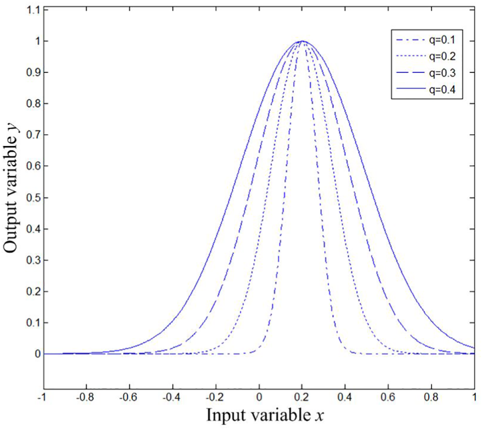
Curves of Gaussian kernel function.

Different kernel functions possess different nature. In this work, the kernel functions with different advantages are combined to make the prediction model more reasonable.

A mixed kernel function is constructed using Gaussian kernel function and polynomial kernel function. If the weight of the Gaussian kernel function is $\gamma$ and the weight of the polynomial kernel function is $(1-\gamma )$ , then

$$K({\mathit{x}}_i,{\mathit{x}}_j)=\gamma K_{\mathrm{Gauss}}+(1-\gamma )K_{\mathrm{Ploy}}$$

(8)

The curves of mixed kernel function are presented in Figure 5. It can be concluded that for x < −0.2 and x > 0.6, all output variables change.

Figure 5.

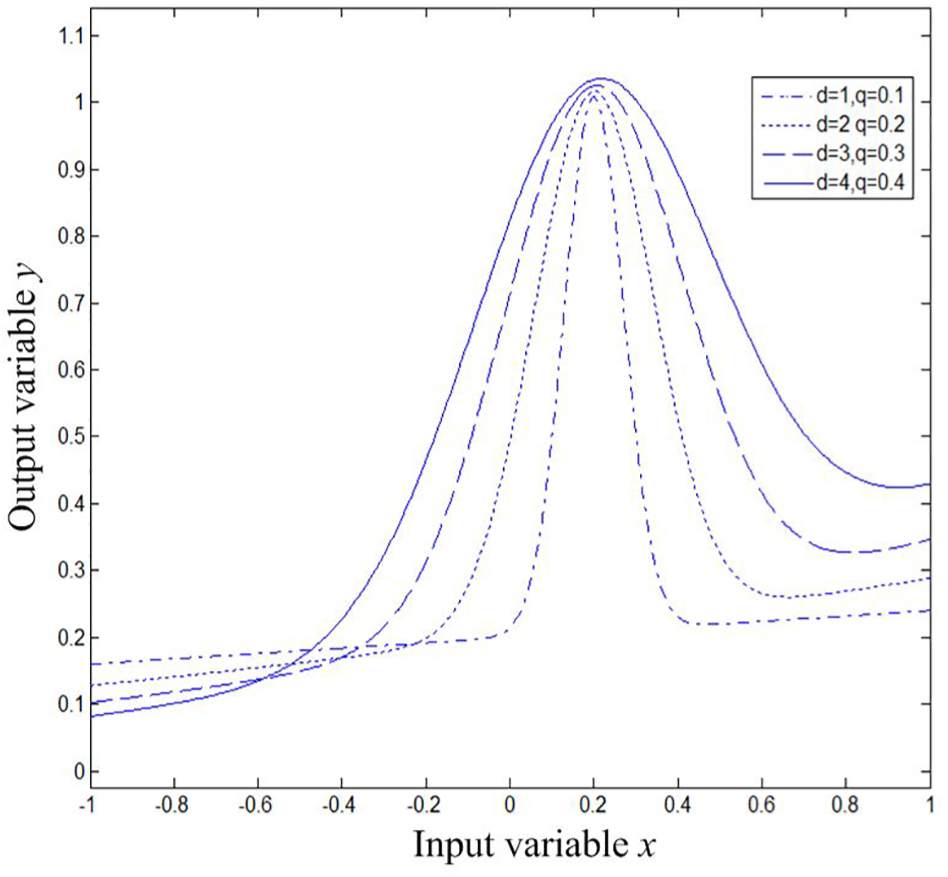
Curves of mixed kernel function.

Training set optimization

In the learning process, the samples, which are most beneficial to improve the performance of learning machine, are selected from the original training set samples to train the prediction model; hence, the number of training samples is significantly reduced as well as the complexity of the model sample is lowered. This process is termed as active learning. The SVM based on active learning can select the training samples with less quantity and high quality; therefore, the performance of learning machine is enhanced.

The sample presents a point set distribution in the space. For the sample, the probability of appearing on the edge of the point set is small. From information theory, it is well known that the amount of information carried by these kinds of sample points is large. The number of sample points on the point set edge is far less than the total number of samples. Therefore, the training of SVM through these kinds of sample points can greatly improve the algorithm speed. The convex hull vertices of the set of sample points are typical edge points, and the optimization of training set is also transformed into the problem of finding the set of convex hull vertices of the original training sample.^18,19

Set $\mathit{G}=\{{\mathit{x}}_1,{\mathit{x}}_2,\dots ,{\mathit{x}}_l\},{\mathit{x}}_j\in \mathit{G}$ , the equation is given by

$$\begin{array}{c}\multicolumn{1}{c}{{\mathit{x}}_j=\sum _{i=1,i\ne j}^l{\lambda }_i{\mathit{x}}_i}\\ \multicolumn{1}{c}{\sum _{i=1,i\ne j}^l{\lambda }_i=1,{\lambda }_i⩾0,i=1,2,\dots ,l}\end{array}$$

(9)

If the above equation is unsolvable, ${\mathit{x}}_j$ is the vertex of the convex hull of G. Now, mapping it to the feature space using the kernel function $K(x,y)$ , we can obtain

$$\{\begin{array}{c}({\mathit{P}}^{\mathrm{T}}\mathit{P})\mathit{x}=\mathit{e}\hfill \\ \multicolumn{1}{c}{\sum _{i=1}^l{\lambda }_i=1}\\ \multicolumn{1}{c}{{\lambda }_i⩾0}\end{array}$$

(10)

The feature sample point of ${\mathit{x}}_j$ is the vertex of the convex hull, which contains the characteristic sample points of all elements of G and itself. In the above formula, $e=[1,1,\dots ,1{]}_{1\times l}^{\mathrm{T}}$ and

$${\mathit{P}}^{\mathrm{T}}\mathit{P}=\left[\begin{array}{c}1+K({\mathit{x}}_1,{\mathit{x}}_1)+K({\mathit{x}}_j,{\mathit{x}}_j)-2K({\mathit{x}}_1,{\mathit{x}}_j),\dots ,1+K({\mathit{x}}_1,{\mathit{x}}_n)+K({\mathit{x}}_j,{\mathit{x}}_j)-K({\mathit{x}}_1,{\mathit{x}}_j)-K({\mathit{x}}_n,{\mathit{x}}_j)\hfill \\ \multicolumn{1}{c}{1+K({\mathit{x}}_1,{\mathit{x}}_2)+K({\mathit{x}}_j,{\mathit{x}}_j)-K({\mathit{x}}_1,{\mathit{x}}_j)-K({\mathit{x}}_2,{\mathit{x}}_j),\dots ,1+K({\mathit{x}}_1,{\mathit{x}}_n)+K({\mathit{x}}_j,{\mathit{x}}_j)-K({\mathit{x}}_1,{\mathit{x}}_j)-K({\mathit{x}}_n,{\mathit{x}}_j)}\\ \multicolumn{1}{c}{\dots }\\ \multicolumn{1}{c}{1+K({\mathit{x}}_1,{\mathit{x}}_n)+K({\mathit{x}}_j,{\mathit{x}}_j)-K({\mathit{x}}_1,{\mathit{x}}_j)-K({\mathit{x}}_n,{\mathit{x}}_j),\dots ,1+K({\mathit{x}}_n,{\mathit{x}}_n)+K({\mathit{x}}_j,{\mathit{x}}_j)-2K({\mathit{x}}_n,{\mathit{x}}_j)}\end{array}\right]$$

(11)

Parameter optimization of SVM

The establishment of the prediction model is the first step, and the optimization of parameters has an immense influence on the model.^20–22 In this work, cross-validation method is carried out to optimize c and g in the prediction model (where c is the error penalty factor and g is the Gaussian kernel parameter; they are coefficients). Cross-validation optimization is an excellent statistical optimization method, ²³ and the basic idea behind it is to divide the initial data into two groups: training sets and validation sets. First, the training set is used to develop the prediction model, and then the model is employed to predict the test set. Finally, the prediction accuracy of the model is utilized as the evaluation performance index. This method can effectively avoid the occurrence of over-learning or under-learning and can obtain an ideal prediction accuracy for the prediction of a test set. In literature, several types of cross-validation parameter optimization methods can be found.

According to the leave-one-out cross-validation method, all samples of original N sample are used as verification sets, while the rest of the N− 1 samples are employed as training sets, and thus the N models are obtained. The mean value of the prediction accuracy of the N models is used as the prediction precision. Because almost all samples in the set are used to train the model, it is closest to the distribution of the original sample. However, the obvious shortcomings, large modeling number, slow speed, and high cost are the main disadvantages of this process.

According to K-fold cross-validation method, the original data are divided into K groups, where each of them is a validation set, and the rest of the K−1 subset data are used as training sets. In this case, the average value of the prediction accuracy of the K model is used as the performance index of the prediction model. The method can effectively avoid the occurrence of over-learning or under-learning; hence, the final result displays high credibility.

Considering the accuracy and speed of the prediction model, the K-fold cross-validation method is applied in our work. The optimal parameters are obtained through the grid search of c and g, thus improving the precision of the model as well as reducing the time required for calculation.

In the present problem, the main steps are developed as follows:

1. The grinding data are divided into K groups, where each of them is a verification set, while the remaining K−1 groups are used as training sets. Finally, the K models are obtained.

2. After dividing c and g into grids, the average value of the prediction accuracy of the final verification set of K models is used as the prediction precision of the LSSVM prediction model. The combination of parameters that manifested the highest precision of prediction is selected as the final optimization parameters.

Online prediction model of CRV

The prediction model can achieve accurate online prediction based on the LSSVM theory, error correction theory, incremental theory, and the theory of mixed kernel function. The online training of SVM can timely import processing data, eliminate obsolete data, and update the model in time. The model is suitable for actual machining processes, and the excellent error correction ability of this model significantly improves the prediction accuracy.

Error correction

Using the difference between measured historical CRV and the predicted value, the error of the new samples can be estimated. The equation of the model is described below

$$Y(k+1)=y(k+1)+\mathrm{\Delta }(k+1)$$

(12)

where $y(k+1)$ is the predicted value of CRV, $\mathrm{\Delta }(k+1)$ is the predicted error of CRV, and $Y(k+1)$ is the predicted value that has been corrected.

The steps of the algorithm are explained below:

1. Build a rough prediction model and predict $y(k+1)$ ;

2. Build a prediction model of the error of CRV and predict the error of $\mathrm{\Delta }(k+1)$ ;

3. Using the predicted value of the error of $\mathrm{\Delta }(k+1)$ in the second step, correct the predicted value of $Y(k+1)$ in the first step.

Online prediction model of CRV

Prediction of CRV can remarkably improve the accuracy of machined workpieces as well as the degree of automation of grinding process. The workpiece diameter, buffing allowance, temperature, wheel speed, and workpiece speed are the main factors that affect the CRV in any grinding process.

The algorithm for prediction and compensation value feedback control of CRV is depicted below:

1. The pre-processing of original data and the construction of sample data include the elimination of gross error, the search of mean data, and the normalization of data.

2. The convex hull vertex set algorithm is employed to find the support vector.

3. The set of training samples for the prediction model is $\{({\mathit{x}}_i,{\mathit{y}}_i)\}$ , where, ${\mathit{x}}_i$ is the input value and ${\mathit{y}}_i$ is the CRV. ${\mathit{x}}_i$ is a five-dimensional vector and composed of five sets of parameters: workpiece diameter, buffing allowance, temperature, wheel speed, and workpiece speed.

4. The parameter optimization method is used to optimize the prediction model to achieve optimal parameters.

5. Using the prediction model, the predicted value of CRV and the predicted value of the error of CRV are found as ${\hat{y}}_{k+1}$ and ${\hat{\mathrm{\Delta }}}_{k+1}$ , respectively. ${\hat{Y}}_{k+1}$ is the predicted CRV that is corrected by ${\hat{y}}_{k+1}$ and ${\hat{\mathrm{\Delta }}}_{k+1}$ . If ${\hat{Y}}_{k+1}$ exceeds the normal compensation range $\pm \lambda$ , the system will alarm. If ${\hat{Y}}_{k+1}$ is in the normal compensation range $\pm \lambda$ , the system needs to be compensated, thus a closed-loop feedback control system is formed through the adjustment of signal points using the active measurement control instrument. The flowchart of the prediction and compensation value feedback control of CRV is illustrated in Figure 6.

Figure 6.

Prediction and compensation value feedback control of CRV.

In the grinding process, after predicting CRV, it should be judged whether the value transcends the upper and lower limits or not. If yes, the system will alarm; otherwise, the compensation and feedback control will work. Figure 7 explains the relationship between CRV and the limits.

Figure 7.

Relationship between CRV and the limits.

Experiment and analysis

The grinding experiment is carried out on the MGB1320 precision semi-automatic grinder, where the measuring instrument is a self-developed control instrument. The setup of the grinding process is exhibited in Figure 8.

Figure 8.

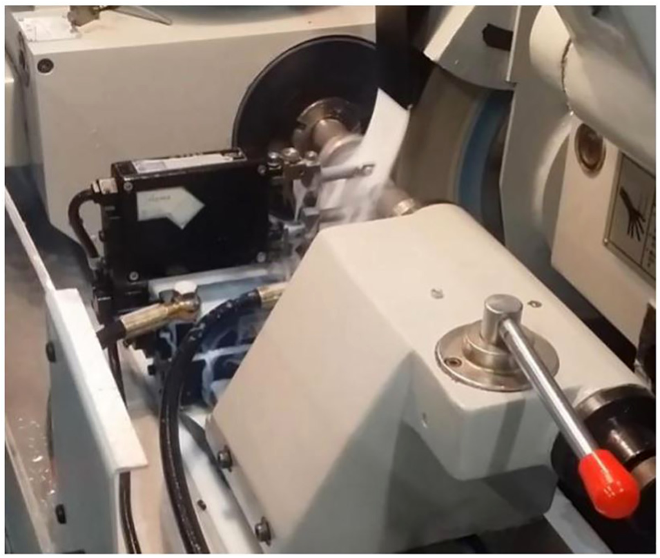
Grinding process setup.

Using the single-factor experimental scheme, 20 workpieces are processed in each group. After processing, the sizes of the workpieces are measured using a pneumatic gauge. During the measurement process, five measuring points are selected for each workpiece and the average of the remaining three values is taken as the real size after removing the maximum and minimum values. Furthermore, by calculating the difference between the measured value and the nominal value, the influence of the accidental factors in the measurement process is removed. The sampling error is then averaged, and at the same time, the average of the measurement size and the compensation value are calculated to fit the real grinding process modeling data.

When a single factor is considered, the prediction model is developed separately based on workpiece diameter, buffing allowance, temperature, wheel speed, and workpiece speed. In contrast, when the comprehensive factors are considered, the prediction model to predict CRV is created separately on the basis of comprehensive factors. The program is compiled with MATLAB. Table 1 displays the cylindrical grinding experimental results and the predicted CRV. The second to sixth columns are the influencing factors, the seventh column is the actual value of the compensation, the eighth column denotes the predicted value of the single-factor training model compensation value, and the ninth column presents the predicted value of the multi-factor-weighted training model compensation value.

Table 1.

Test results and prediction of CRV.

N	Workpiece diameter (mm)	Buffing allowance (μm)	Temperature (°C)	Wheel speed (m/s)	Workpiece speed (r/min)	Measured CRV (μm)	Predicted CRV (single factor) (μm)	Predicted CRV (multi-factor) (μm)
1	50	8	20	25	150	−2.7	−2.58	−2.62
2	60	8	20	25	150	−2.2	−2.13	−2.25
3	70	8	20	25	150	−1.7	−1.83	−1.81
4	80	8	20	25	150	−1.1	−1.26	−1.29
5	90	8	20	25	150	−0.7	−0.77	−0.69
6	100	8	20	25	150	−0.2	0.01	−0.03
7	110	8	20	25	150	0.5	0.69	0.69
8	120	8	20	25	150	1.3	1.46	1.46
9	130	8	20	25	150	2.1	2.27	2.28
10	140	8	20	25	150	3.2	3.29	3.13
11	150	8	20	25	150	4.1	4.25	4.22
12	100	6	20	25	150	−1.7	−1.49	−1.58
13	100	7	20	25	150	−0.8	−0.91	−0.77
14	100	8	20	25	150	−0.2	−0.03	−0.03
15	100	9	20	25	150	0.3	0.23	0.27
16	100	10	20	25	150	0.3	0.41	0.34
17	100	11	20	25	150	0.4	0.35	0.47
18	100	12	20	25	150	0.2	0.22	0.19
19	100	8	15	25	150	−1.5	−1.36	−1.32
20	100	8	17	25	150	−0.9	−0.79	−0.83
21	100	8	19	25	150	−0.4	−0.61	−0.31
22	100	8	21	25	150	−0.1	−0.09	0.03
23	100	8	23	25	150	0.6	0.72	0.74
24	100	8	25	25	150	1.2	1.41	1.32
25	100	8	27	25	150	1.8	1.93	1.89
26	100	8	29	25	150	2.5	2.44	2.43
27	100	8	31	25	150	3.1	2.96	2.98
28	100	8	20	20	150	0.2	0.23	0.33
29	100	8	20	22	150	0.2	0.09	0.12
30	100	8	20	24	150	0.1	−0.07	−0.03
31	100	8	20	26	150	0.3	0.23	0.19
32	100	8	20	28	150	0.9	0.73	0.77
33	100	8	20	30	150	1.6	1.45	1.52
34	100	8	20	32	150	2.4	2.55	2.41
35	100	8	20	34	150	3.5	3.46	3.43
36	100	8	20	36	150	4.6	4.47	4.53
37	100	8	20	25	100	0.5	0.43	0.49
38	100	8	20	25	120	0.4	0.33	0.32
39	100	8	20	25	140	0.2	0.29	0.10
40	100	8	20	25	160	−0.1	−0.25	−0.18
41	100	8	20	25	180	−0.4	−0.49	−0.52
42	100	8	20	25	200	−0.7	−0.88	−0.91
43	100	8	20	25	220	−1.2	−1.36	−1.35
44	100	8	20	25	240	−1.9	−1.79	−1.82
45	100	8	20	25	260	−2.5	−2.39	−2.33

CRV: compensation regulation value.

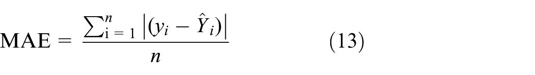
The prediction model of compensation value is evaluated using mean absolute error (MAE) and root mean square error (RMSE).

MAE can be formulated as

$$\mathrm{MAE}=\frac{\sum _{\mathrm{i}=1}^n|(y_i-{\hat{Y}}_i)|}{n}$$

(13)

The equation of RMSE is presented below

$$\mathrm{RMSE}=\sqrt{\frac{\sum _{\mathrm{i}=1}^n{(y_i-{\hat{Y}}_i)}^2}{n}}$$

(14)

where $y_i$ is the measured value and ${\hat{Y}}_i$ is the predicted value.

It is observed that the smaller values of MAE and RMSE yielded higher accuracy and stability of the prediction model.

When the grinding parameter settings within the sample are employed to predict the compensation value of the cylindrical grinding, the parameters of the single-factor training model are optimized. The cross-validation parameters are presented in Table 2.

Table 2.

Model parameters and prediction accuracy assessment of the model under single factor.

Single factor	Model parameters		Prediction accuracy
	c	g	MAE (μm)	RMSE (μm)
Workpiece diameter	16	0.125	0.1382	0.1452
Buffing allowance	103.9683	0.25	0.1057	0.1225
Temperature	2.8284	0.25	0.1256	0.1392
Wheel speed	2.8284	0.6156	0.1133	0.1244
Workpiece speed	4	0.5	0.1144	0.1205

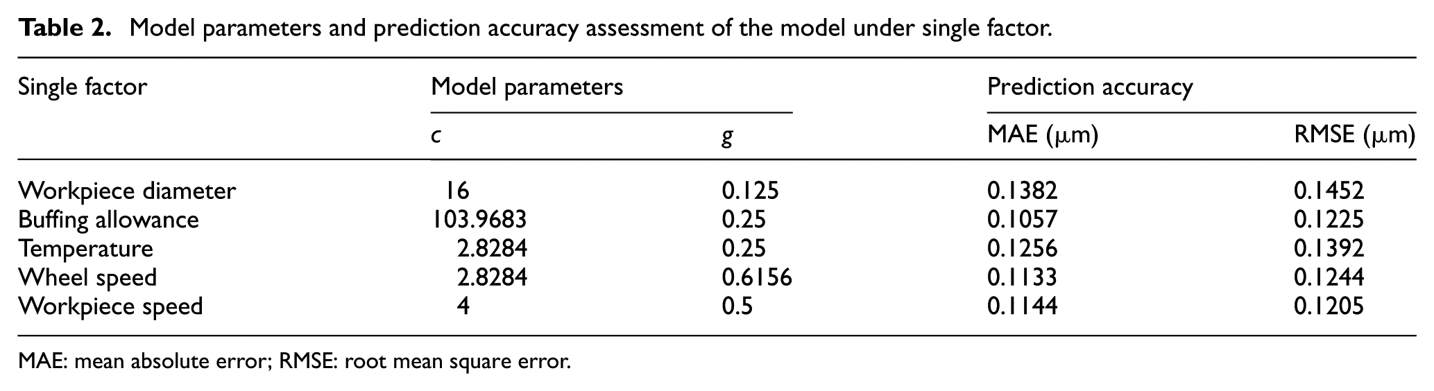
MAE: mean absolute error; RMSE: root mean square error.

Figure 9 compares the predicted CRV and the measured CRV values for the single-factor model. The abscissa represents the amount of each type of influencing factor and the ordinate describes the compensation value.

Figure 9.

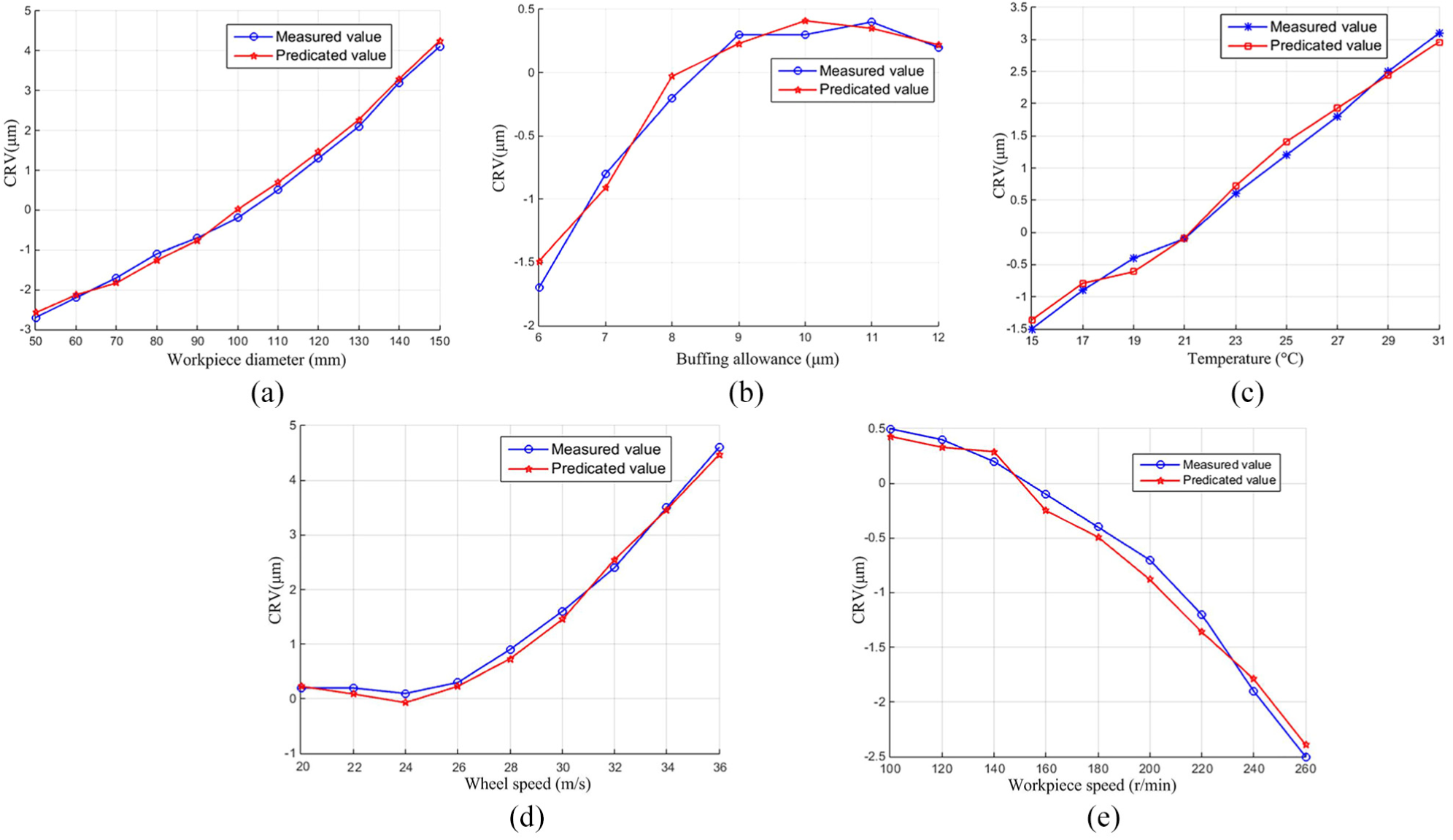
Comparison between predicted and measured CRV for the single-factor model: (a) workpiece diameter, (b) buffing allowance, (c) temperature, (d) wheel speed, and (e) workpiece speed.

The prediction model of compensation value using a single factor has high credibility to local problems. Table 2 presents the prediction accuracy assessment of the model under a single factor.

In our experiment, the online error compensation LSSVM model is employed for the prediction of CRV, and the values of c and g are obtained as 13.9288 and 0.3789, respectively. It can be seen from Figure 10 that the optimization result (three-dimensional view) of the model is established using 45 sets of data training in the sample. The horizontal axis and the vertical axis represent ${\log }_{2}c$ and ${\log }_{2}g$ , respectively. The vertical axis denotes the corresponding prediction accuracy. RMSE is chosen as the evaluation criterion in this case.

Figure 10.

Schematic diagram of parameter optimization results of cross-validation model.

The eighth column of Table 1 describes the predicted values of compensation value under the multi-factor-weighted prediction model. In this case, the values of MAE and RMSE are found as 0.1027 and 0.1154 μm, respectively. Figure 11 compares the predicted and the measured values of compensation value. The abscissa represents the number of groups, whereas the ordinate signifies the compensation value.

Figure 11.

Comparison between predicted and measured CRV of the sample.

In order to verify the feasibility of the training set optimization method, the factors are reset separately as follows: workpiece diameter: 50–150 mm with a step size of 5, buffing allowance: 6–12 μm with a step size of 1, temperature: 15°C–31°C with a step of 1, wheel speed: 20–36 m/s with a step of 1, and workpiece speed: 100–260 r/min with a step of 10. Then, 80 sets of factors’ data and the actual compensation value are obtained by cylindrical grinding experiments.

On the basis of comprehensive factors analysis, the prediction model to predict CRV is created with the training sets, which are optimized by convex hull vertex algorithm. In the other creating process, we do not optimize the training sets. For clarity, these two approaches are expressed as SVM-O and SVM. As shown in Table 3, the MAE and RMSE of SVM-O are similar to those of SVM. Moreover, it can be seen that the calculation time of SVM-O is significantly shorter than the time of SVM in this comparison.

Table 3.

Comparison of prediction accuracy and calculation time.

Approach	MAE (μm)	RMSE (μm)	Calculation time (s)
SVM	0.1032	0.1158	12.32
SVM-O	0.1030	0.1164	8.16

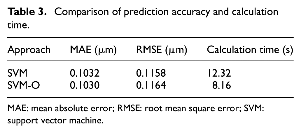
MAE: mean absolute error; RMSE: root mean square error; SVM: support vector machine.

However, when the in-sample data are utilized to verify the accuracy of the model, over-learning, weak generalization, and poor promotion capabilities are noted, thus making it difficult to ensure the usability of the model. Using the prediction model of the compensation value and the grinding parameters outside the sample, the cylindrical grinding machining experiment is performed to analyze the prediction accuracy of the model as well as to determine whether the prediction accuracy attain the requirements of the active measurement controller. The grinding experiments are carried out in eight groups with sample outside. Table 4 depicts the measured and the predicted values of compensation value for the grinding process.

Table 4.

Measured and predicted values of the CRV for the grinding process.

N	Workpiece diameter (mm)	Buffing allowance (μm)	Temperature (°C)	Wheel speed (m/s)	Workpiece speed (r/min)	Measured CRV (μm)	Predicted CRV (μm)
1	60	9	20	25	110	−1.1	−1.19
2	70	7	24	28	130	−1.5	−1.41
3	80	10	25	30	150	−0.8	−0.72
4	120	11	30	22	120	2.5	2.69
5	90	10	26	33	180	−0.3	−0.39
6	100	11	19	20	200	0.3	0.43
7	110	7	20	22	230	−3.0	−2.89
8	130	8	25	28	200	1.1	0.98

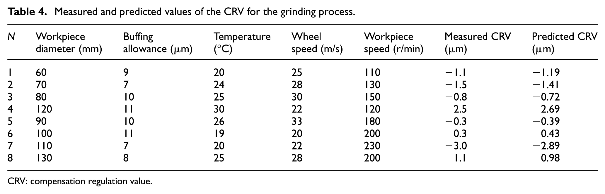
CRV: compensation regulation value.

When the prediction model predicts the compensation value under the external sample grinding parameter setting, the values of MAE and RMSE are calculated as 0.1125 and 0.1174 μm, respectively. Figure 12 presents the comparison of the predicted and measured values of compensation value with sample outside.

Figure 12.

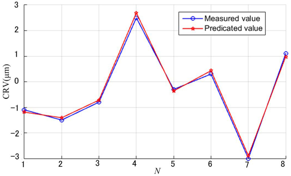
Comparison between predicted and measured values of the sample.

Applying the prediction model of compensation value to the cylindrical grinding error feedback compensation system, the setting of the grinding compensation value is controlled online for a number of cylindrical workpieces with the size of 100 mm, buffing allowance of 10 μm, temperature of 20°C, workpiece speed of 150 r/min, and wheel speed of 28 m/s. Figure 13 illustrates the size distribution of batch workpieces, and it can be identified that the batch workpiece processing accuracy fulfilled the requirements. Moreover, in comparison with unused compensation value, the compensation control is significantly improved.

Figure 13.

Size distribution map of batch workpieces.

Conclusion

To set CRV artificially in any grinding and active measurement process, a large amount of randomness and poor real-time problem can be noted. In this research, the prediction theory for the grinding process is studied, and the prediction model of CRV is developed based on the LSSVM theory, error correction theory, incremental theory, and the theory of mixed kernel function. The results demonstrated high prediction accuracy for CRV of the workpieces. Applying the prediction model to the grinding process, a timely feedback control system is developed to realize the automatic adjustment of process parameters. The obtained results can be utilized to improve the efficiency of machining accuracy as well as to enhance the intelligence level of the grinding process.