Sage Journals: Discover world-class research

Abstract

Impulsive noise, generated by inverters and other equipment used in the field, tends to easily enter test channels in scenarios where continuous frequency conversion signals are employed to test the frequency response of electrohydraulic proportional valves. Interference caused by such noise reduces the signal-to-response ratio of response signals, thereby influencing the accuracy of the frequency response of proportional valves. To address this concern, in this article, an integrated filtering method that combines ensemble empirical mode decomposition with median filtering is proposed. The proposed method first preprocesses the response signals of the systems and subsequently obtains frequency-response diagrams using fast Fourier transforms. Simulation results demonstrate that the proposed method reduces the root mean square error associated with the amplitude–frequency characteristic curves of the proportional directional valve considered from 2.1 to 0.3, whereas that associated with phase–frequency characteristic curves is reduced from 78.0 to 1.4 with signal-to-noise ratios in the high-frequency band being of the order of –20 dB. Experimental results also reveal that the proposed method reduces the root mean square error of the amplitude–frequency characteristic curves of the proportional directional valve by 52.5% and that of the phase–frequency characteristic curves by 71.2%.

Keywords

Ensemble empirical mode decomposition median filtering frequency-response testing impulsive noise electrohydraulic proportional valve

Introduction

Electrohydraulic proportional valves are used extensively in numerous industries—such as metallurgy, marine, and automobile¹—and constitute the core components of proportional control systems. Consequently, the frequency response of these valves often determines the performance of proportional control systems. Accurate determination of the frequency response of electrohydraulic proportional valves is therefore important. However, employing continuous frequency conversion signals to test the frequency response of electrohydraulic proportional valves often involves interference caused by impulsive noise generated by devices, such as inverters, present at the test site. These impulsive noise signals superimpose and enter the test channel through the power supply terminal and space radiation, thereby significantly reducing the signal-to-noise ratio (SNR) over time t. The amplitudes of these noise signals are significantly larger than those of pure signals generated during this interval.² Owing to the influence of impulsive noise, the test signal typically becomes nonstationary. To rectify this problem, Huang et al.³ proposed a technique—called empirical mode decomposition (EMD)—that decomposes signals into several physically meaningful intrinsic mode functions (IMFs) along with a residual trend from high to low frequencies.⁴ An advantage of EMD is that the signal is self-adaptive and well suited for handling nonstationary signals.³ However, there exists a serious concern with regard to mode mixing in EMD, which occurs when signals contain intermittent components, such as pulses.^5–8 To tackle this problem, Wu and Huang⁹ proposed the ensemble empirical mode decomposition (EEMD) technique based on the statistical properties of white noise. EEMD enhances EMD in the form of an effective adaptive filter, the use of which causes addition of white noise to signals to help smoothen intermittent components, such as pulses, thereby proving helpful with regard to EMD data analysis.^10,11 The basic principle underlying EEMD is addition of white noise to signals being decomposed, thereby ensuring an even distribution of noise across the entire time–frequency space. When a signal is added to a uniformly distributed white-noise background, signal components of different scales get automatically distributed in accordance with an appropriate reference scale. After multiple rounds of averaging, the noise types tend to cancel each other, and the ensemble mean is considered the final result.^9,12 Currently, EEMD is widely employed in signal-processing applications. Patel et al.¹³ proposed a denoising method based on principal component analysis and EEMD that demonstrates an optimum denoising effect on contaminated electroencephalogram signals. Mariyappa et al.¹⁴ proposed a denoising method based on independent components analysis and EEMD of multi-channel magnetocardiography signals that is capable of obtaining signals with high SNRs.¹⁴ Based on the EEMD law of white noise, Zhang et al.¹⁵ proposed a method that determines the standard deviation in signal noise after performing EEMD on noisy signals to solve the problem of noise decreasing the accuracy of modal-parameter identification in hydraulic structures. Their proposed method improves the denoising method that combines EEMD and wavelet threshold.

The methods described above are employed extensively in pattern recognition and biomedical signal-processing applications. Usually, these fields do not require consideration of the impact of inverter usage. Nevertheless, variable-frequency drives are often used at test sites for numerous reasons, such as energy conservation and low heat dissipation cost, and inverters form a vital component of variable-frequency drives. It is therefore necessary to consider reduction of the impulse noise produced by inverters.

To address the above concern, this article proposes an integrated filtering method that combines EEMD and median filtering (EEMD–MF) to filter out impulse noises from the response signals of proportional directional valves. In the proposed method, EEMD is first used to separate high-frequency noise from test signals and subsequently amplify the amplitude of useful signals to improve the SNR of test signals. Then, MF is applied to further eliminate any impulse noise remaining within the test signal.

Basic principle underlying EEMD-MF

Principle of EEMD

EEMD is an improved decomposition method based on EMD. Its underlying procedure can be described as follows:^9,12

Add a white-noise series to a target signal.

Decompose the target signal with added white noise into IMFs using the EMD approach. When employing EEMD to decompose the target signal, the number of IMFs needs to be determined. The following points explain the corresponding methodology.

If the total number of IMFs is too small to accurately decompose the target signal, the accuracy of model aliasing component identification may be adversely affected. Conversely, certain components may get excessively extracted in such a manner that the accuracy of model aliasing component identification is not affected. When data contain pure white noise, the total number of IMFs obtained in the dataset approaches a value close to log₂N, with N being the total number of data points; otherwise, the total number of IMFs is less than log₂N. Thus, the maximum number of IMFs can be specified as (log₂N– 1) for the purpose of this study. In addition, if the residue value follows a monotonic function prior to the number of IMFs being equal to its maximum value, the EEMD process can be terminated.⁹

Repeat the previous step as many times as necessary, while using a different white noise series during each repetition.

Obtain the ensemble mean using equation (1) as the final result

w_{i} = \frac{\sum_{j = 1}^{L} w_{i, j}}{L}

(1)

where w_i,j denotes the ith IMF of the jth repetition; L represents the total number of repetitions; and w_i is ith IMF of the final result.

Principle of MF

The basic principle underlying MF involves browsing through the signal series using a window of a given length. To obtain the median, the series within the window are sorted according to size. Subsequently, the centered sample value in the window is replaced by the median. Assuming that a window of length M slides over a sample series and contains x = {x₁, x₂, …, x_M} by sorting M numbers by size, the median of the sequence can then be defined as

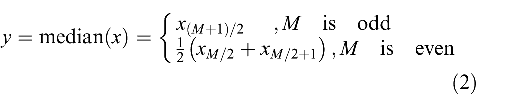
y = median (x) = {\begin{matrix} x_{(M + 1) / 2} & , M is odd \\ \frac{1}{2} (x_{M / 2} + x_{M / 2 + 1}) & , M is even \end{matrix}

(2)

where M denotes the MF window length. In general, the larger the window length, the better the denoising effect. Nevertheless, only one available dataset is finally obtained after all the sampled data in the window are filtered. Hence, when the sampling frequency is fixed, a long window implies that more sampled data need to be filtered out to ultimately obtain available data and that a short window cannot reduce the noise interference. Therefore, the sampling frequency, available data, and denoising effect must be considered when determining the window length. The minimum length of the window should contain at least one impulsive noise and several valid sampling signals nearby. The window length is, ultimately, a compromise.

Principle of EEMD–MF

The proposed EEMD–MF is an integrated filtering method that combines the EEMD and MF techniques. The basic procedure employed when performing EEMD–MF is as follows:

The signal y(t) to be processed is first decomposed into IMFs using EEMD.

IMFs that undergo mode mixing are identified by the cross–correlation coefficient between y(t) and IMFs. The IMF corresponding to the first local minimum of the cross–correlation coefficient is marked as imf_k, while imf_k₊₁ undergoes mode mixing¹⁶

R (y, im f_{j}) = \frac{\sum_{i = 1}^{N} [y (t) - \bar{y}] [im f_{j} (t) - \bar{im f_{j}}]}{\sqrt{\sum_{i = 1}^{N} {[y (t) - \bar{y}]}^{2}} \sqrt{\sum_{i = 1}^{N} {[im f_{j} (t) - i \bar{m f_{j}}]}^{2}}}

(3)

where imf_j denotes the jth IMF, N denotes the number of sampling points, and

\bar{y} = \frac{1}{N} \sum_{i = 1}^{N} y (t), \bar{im f_{j}} = \frac{1}{N} \sum_{i = 1}^{N} im f_{j} (t)

The first (k) IMFs are discarded, and the signal is reconstructed by combining other IMFs with the residual signal.

With the aim of obtaining a denoised signal, the signal—post reconstruction—is filtered using MF.

Simulation analysis of EEMD–MF

Impulsive noise model

An impulsive noise can be expressed as follows¹⁷

u_{p} (k) = u (k) b (k)

(4)

where u_p(k) denotes the impulsive noise, b(k) represents a random binary series that describes the presence or absence of impulsive noise, u(k) denotes a random variable that describes the amplitude of the impulsive noise, and k represents discrete time. An impulsive noise, u_p(k), can be modeled, as described in Figure 1, as the output of a channel filter excited by an amplitude-modulated random binary sequence, expressed as

u_{p} (k) = \sum_{i = 1}^{P - 1} h (i) u (k - i) b (k - i)

(5)

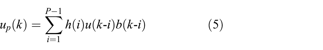
where h(k) denotes the impulse response of a filter that models the duration and shape of each impulse.

Figure 1.

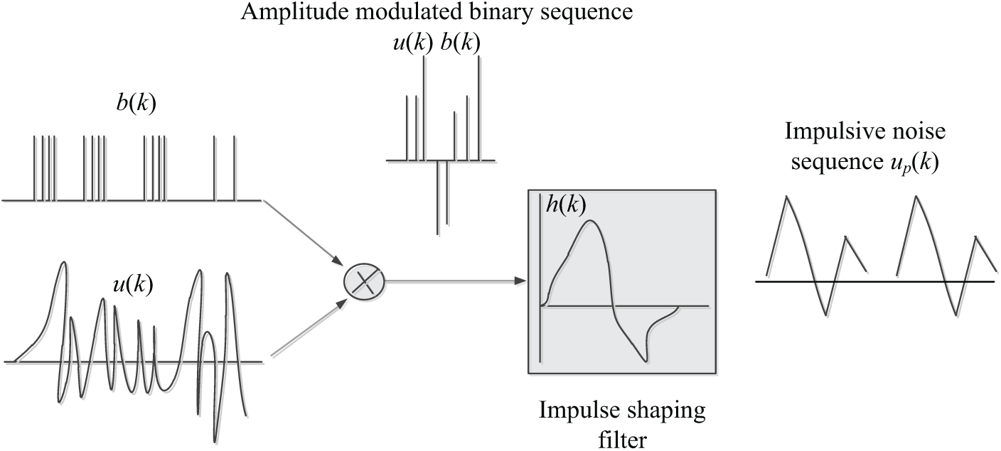
Impulsive-noise modeled as output of filter excited by amplitude-modulated binary sequence.

The noise collected at the project site is depicted in Figure 2. Figure 2(a) and (b), respectively, show the amplitude and power spectrum of the impulsive noise. Signals with amplitude greater than 0.07 are considered impulsive noise. The number of impulsive noise signals is denoted by N₁, and the number of sampling points N₂ is counted. Subsequently, the probability of impulsive noise is determined as N₁/N₂ = 0.23. The observed variance in the impulsive noise amplitude is 0.026. Finally, the impulsive noise u_p(k) was obtained using the method described in Figure 1.

Figure 2.

(a) Impulsive noise data collected at project site and (b) its power spectrum.

Simulation analysis

As depicted in Figure 3, under dynamic conditions, if the influence of nonlinear factors, such as coulomb friction, is ignored, proportional directional valves can be considered equivalent to spring–mass–damper second-order vibrating systems comprising reset springs and viscous friction of slide valves. In this study, a second-order system was, therefore, considered as the test object to analyze the denoising effect of EEMD–MF.

Figure 3.

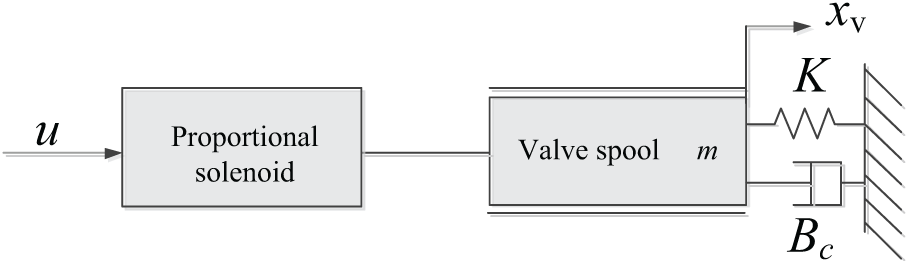
Equivalent model for proportional directional valve.

The transfer-function model of the said second-order system can be expressed using equation (6)

G (s) = \frac{X_{v} (s)}{U (s)} = \frac{K}{m s^{2} + B_{c} s + K}

(6)

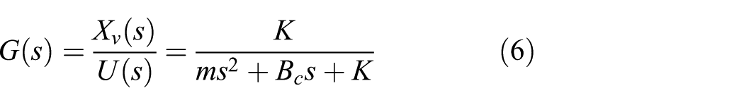
where m denotes spool mass, K denotes the stiffness of the reset spring, and B_c denotes the viscous damping coefficient for the proportional valve. The value of B_c reflects the relationship between fluid viscosity and spool speed, while the size of the damper relates to the fluid viscosity and valve structure. The value of B_c can be obtained experimentally.

The transfer function model of the proportional directional valve can be obtained in accordance with the values of the spool mass, reset spring stiffness of typical products provided by the manufacturer, and viscous damping coefficient obtained via experiments, as described in equation (7)

G (s) = \frac{156.25}{s^{2} + 20 s + 156.25}

(7)

A chirp signal, measuring 4 V in amplitude and having frequency lying in the range of 0.1–8 Hz, was provided as input to the second-order system, and the sampling period was set as 0.001 s. Corresponding response and chirp signals were subsequently collected to obtain system excitation x(k) and response y(k) signals (k = 0, 1, …, n; n represents the maximum number of sampling points). After adding u_I(k) to the second-order system input terminal, the sampling period was set as 0.001 s, and the response signal y_p(k) was collected and subsequently filtered using the proposed EEMD–MF approach as follows:

Twelve IMFs were obtained after y_p(k) was decomposed via EEMD.

While identifying IMFs that undergo mode mixing, imf₅ was identified as one of them. Subsequently, after discarding the first four IMFs, the signal y₁(k) was reconstructed by combining other IMFs with the residual signal (Figure 4).

The length M of the window was assumed to be 15; y₁(k) was filtered via MF, and subsequently, y₂(k) was obtained.

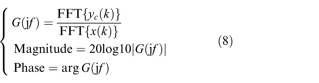
The theoretical value, measurement, and denoising measurement of the second-order system frequency response were calculated using y(k), y_p(k), and y₂(k), respectively, instead of y_c(k) in equation (8); corresponding results are depicted in Figure 5

{\begin{matrix} G (j f) = \frac{FFT {y_{c} (k)}}{FFT {x (k)}} \\ \begin{matrix} Magnitude = 20 \log 10 | G (j f) | \\ Phase = \arg G (j f) \end{matrix} \end{matrix}

(8)

Figure 4.

First four IMFs.

Figure 5.

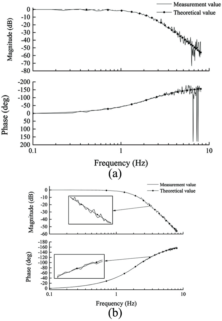
Frequency-response curves of second-order system (a) before denoising and (b) after denoising.

In equation (8), y_c(k) denotes response signals while x(k) represents excitation signals; f represents frequency.

To evaluate the denoising effect of EEMD–MF, the root mean square error (RMSE) was introduced as the evaluation criterion. RMSE values reflect the equivalence between the normal frequency response and frequency response after denoising. The smaller the value of RMSE, the better is the denoising effect considered to be. RMSE can be defined as

RMSE = \sqrt{\frac{\sum_{i = 1}^{N} {[g (i) - G (i)]}^{2}}{N}}

(9)

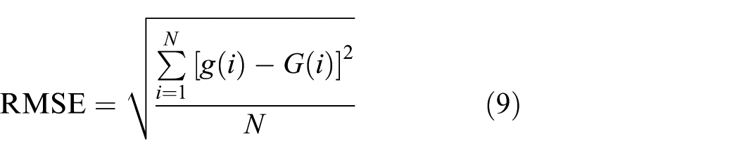
where N denotes the data length while g_i and G_i denote the frequency responses of the system prior to and after denoising, respectively. The RMSE value for the amplitude–frequency characteristics of the second-order system prior to denoising was 2.1, whereas that for phase–frequency characteristics was 78.0. After denoising, corresponding RMSE values for amplitude–frequency and phase–frequency characteristics were 0.3 and 1.4, respectively. These results demonstrate that application of the proposed EEMD–MF method significantly improves the frequency-response-test accuracies for second-order systems.

Experimental validation

A valve test bench was used as the research platform in this study to investigate the denoising effect of EEMD–MF on the frequency-response test data obtained for the electrohydraulic proportional directional valve containing impulse noises.

Experimental system

The experimental system used in this study was powered by a variable-frequency pump station comprising a frequency converter (OMRON 3G3RX-A4185). The stimulation signal for the proportional-directional-valve was input through NI cRIO-9075 (CompactRIO Controller) and NI-9263 (C series vo1tage output module) and subsequently transmitted to the proportional directional valve via a built-in proportional amplifier. Spool position feedback was acquired using NI9201(C series vo1tage input module) and subsequently passed into cRIO-9075. The basic components of the experimental system are depicted in Figure 6(a), whereas the actual experimental setup is depicted in Figure 6(b).

Figure 6.

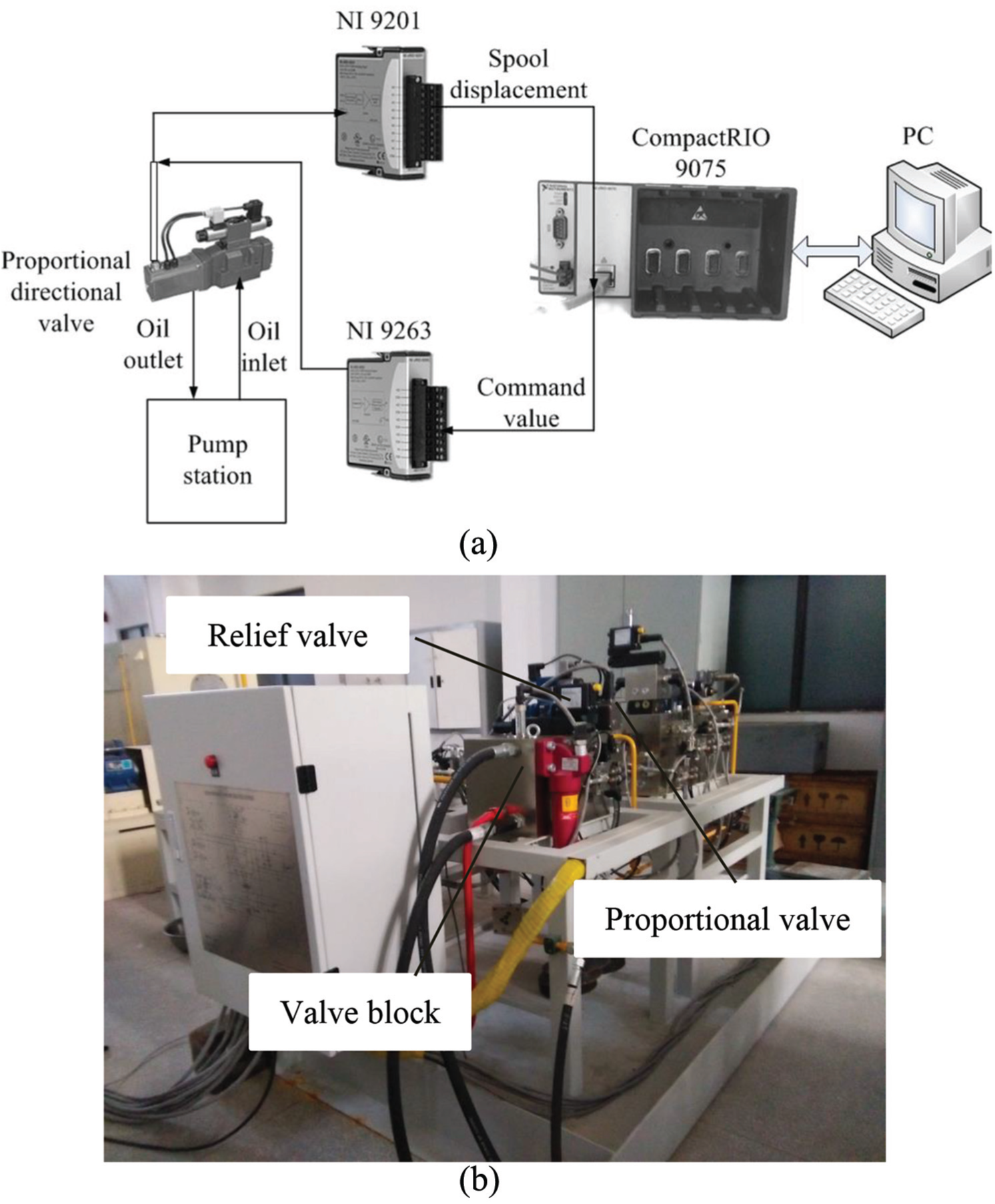
Experimental system and its composition: (a) components of experimental system and (b) actual photograph of experimental system.

Experimental results

The pressure inside the pump station was maintained at 10 MPa, and the inverter frequency was set to 50 Hz. A chirp signal measuring 1 V in amplitude and variable operating frequency of 0.1–50 Hz was provided as input to the electrohydraulic proportional valve.

The sampling period was set as 0.001 s, and the excitation signal x(t) and electrohydraulic proportional-valve-spool feedback y(t) were acquired. Subsequently, X(k) and Y(k) (k = 0, 1, …, n, as described earlier) were obtained, as depicted in Figure 7.

The signal Y(k) was filtered using EEMD–MF as follows:

Fourteen IMFs were obtained after y(k) was decomposed via EEMD.

While identifying IMFs that undergo mode mixing, imf₃ was identified as one of them. After discarding the first two IMFs, the signal Y₁(k) was reconstructed by combining other IMFs with the residual signal (Figure 8).

Length M of the window was assumed to measure 10 units. Y₁(k) was filtered via MF, and subsequently, Y₂(k) was obtained. Frequency response of the electrohydraulic proportional directional valve was calculated using values of Y(k) and Y₂(k) instead of y_c(k) in equation (4). Results obtained are depicted in Figure 9.

Figure 7.

Response and excitation signals for electrohydraulic proportional valve: (a) excitation signal of electrohydraulic proportional valve and (b) response signal of electrohydraulic proportional valve.

Figure 8.

First three IMFs.

Figure 9.

Frequency-response curves for electrohydraulic proportional directional valve (a) before denoising and (b) after denoising.

Evaluation of results

To evaluate the effectiveness of the proposed EEMD–MF method using RMSE, an evaluation criterion must first be defined and appropriately determined. When employing the point-to-point method to measure the frequency response of electrohydraulic proportional directional valves, induced impulsive noises were observed to demonstrate little effect on the response signal, and it was easy to eliminate noise from the response signal, so as to obtain the frequency response with high precision. Consequently, the said point-to-point method was employed in this study to obtain the frequency response of electrohydraulic proportional directional valves as an evaluation criterion. The results obtained are depicted in Figure 10.

Figure 10.

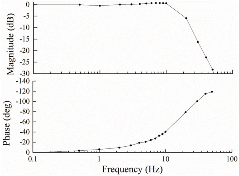
Evaluation criterion for frequency-response curves characterizing electrohydraulic proportional directional valve.

The RMSE values for the electrohydraulic proportional directional valve were calculated for conditions before and after denoising. As can be seen in the figure, the RMSE value for the amplitude–frequency characteristics of the electrohydraulic proportional directional valve prior to denoising was 5.9 while that for the phase–frequency characteristics was 30.9. Following denoising, the RMSE value for the amplitude–frequency characteristics was 2.8 while that for the phase–frequency characteristics was 8.9.

The calculation results obtained in this study indicate that the proposed EEMD–MF method reduces RMSE values for amplitude–frequency and phase–frequency characteristics by 52.5% and 71.2%, respectively. Thus, it is clear that application of EEMD–MF significantly improves frequency-response-test accuracies in the operation of electrohydraulic proportional directional valves.

Conclusion

This article proposed the EEMD–MF method, which combines EEMD with MF, to solve the problem of interference caused by impulsive noise signals that tend to reduce the SNR values of test signals, thereby affecting the frequency response accuracy of proportional directional valves. The results of simulation analysis and tests performed on a typical proportional directional valve demonstrate that the proposed method effectively reduces the RMSE of proportional valve frequency characteristics under conditions of low SNR. The proposed method can therefore be used to filter signals with low SNR values. Furthermore, the proposed EEMD–MF method is more efficient than conventional methods in determining appropriate median-filter window lengths. However, when the sampling rate is low and signal frequency is high, the noise elimination effect of the EEMD–MF method is not ideal. This problem will be addressed in future studies.

Footnotes

Handling Editor: ZW Zhong

Declaration of conflicting interests

The author(s) declared no potential conflicts of interest with respect to the research, authorship, and/or publication of this article.

Funding

The author(s) disclosed receipt of the following financial support for the research, authorship, and/or publication of this article: This research was supported by the National Natural Science Foundation of China (grant number 51765033).

ORCID iD

Yan Qiang

References

Minxia

Dynamic characteristics of large flow rating electro-hydraulic proportional cartridge valve. Chin J Mech Eng 2008; 21: 1.

Zhu

Zhang

Impulsive noise removal based on noise energy distribution in wavelet packet domain. Chin J Sci Instrum 2011; 32: 2071–2078.

Huang

Shen

Long

et al . The empirical mode decomposition and the Hilbert spectrum for nonlinear and non-stationary time series analysis. Proc Roy Soc A Math Phys Eng Sci 1998; 454: 903–995.

Wang

Chen

Dong

Feature extraction of rolling bearing’s early weak fault based on EEMD and tunable Q-factor wavelet transform. Mech Syst Signal Pr 2014; 48: 103–119.

Amirat

Choqueuse

Benbouzid

EEMD-based wind turbine bearing failure detection using the generator stator current homopolar component. Mech Syst Signal Pr 2013; 41: 667–678.

Wang

Zhang

et al . Comparing the applications of EMD and EEMD on time–frequency analysis of seismic signal. J Appl Geophys 2012; 83: 29–34.

Chen

Jeng

Natural logarithm transformed EEMD instantaneous attributes of reflection data. J Appl Geophys 2013; 95: 53–65.

Mariyappa

Sengottuvel

Parasakthi

et al . Baseline drift removal and denoising of MCG data using EEMD: role of noise amplitude and the thresholding effect. Med Eng Phys 2014; 36: 1266–1276.

Huang

NE.

Ensemble empirical mode decomposition: a noise-assisted data analysis method. Adv Adapt Data Anal 2009; 1: 1–41.

10.

Flandrin

Rilling

Goncalves

Empirical mode decomposition as a filter bank. IEEE Signal Process Lett 2004; 11: 112–114.

11.

Huang

NE.

A study of the characteristics of white noise using the empirical mode decomposition method. Proc Roy Soc A Math Phys Eng Sci 2004; 460: 1597–1611.

12.

Lei

Lin

et al . A review on empirical mode decomposition in fault diagnosis of rotating machinery. Mech Syst Signal Pr 2013; 35: 108–126.

13.

Patel

Sengottuvel

Janawadkar

et al . Ocular artifact suppression from EEG using ensemble empirical mode decomposition with principal component analysis. Comput Electr Eng 2016; 54: 78–86.

14.

Mariyappa

Sengottuvel

Patel

et al . Denoising of multichannel MCG data by the combination of EEMD and ICA and its effect on the pseudo current density maps. Biomed Signal Process Control 2015; 18: 204–213.

15.

Zhang

Lian

Liu

An improved filtering method based on EEMD and wavelet-threshold for modal parameter identification of hydraulic structure. Mech Syst Signal Pr 2016; 68–69: 316–329.

16.

Jia

Zhao

Sun

et al . Micro-seismic signal denoising method based on empirical mode decomposition and independent component analysis. Chin J Geophys 2015; 58: 1013–1023.

17.

Vaseghi

Milner

BP.

Speech recognition in impulsive noise. In: Proceedings of the international conference on acoustics, speech, and signal processing, Detroit, MI, 9–12 May 1995, Vol. 1, pp.437–440. New York: IEEE.

Method for filtering proportional valve-frequency-response test data containing impulsive noise

Abstract

Keywords

Introduction

Basic principle underlying EEMD-MF

Principle of EEMD

Principle of MF

Principle of EEMD–MF

Simulation analysis of EEMD–MF

Impulsive noise model

Simulation analysis

Experimental validation

Experimental system

Experimental results

Evaluation of results

Conclusion

Footnotes

Declaration of conflicting interests

Funding

ORCID iD

References