Sage Journals: Discover world-class research

Abstract

A great investment is made in maintenance of machinery in any industry. A big percentage of this is spent both in workers and in materials in order to prevent potential issues with said devices. In order to avoid unnecessary expenses, this article presents an intelligent method to detect incipient faults. Particularly, this study focuses on bearings due to the fact that they are the mechanical elements that are most likely to break down. In this article, the proposed method is tested with data collected from a quasi-real industrial machine, which allows for the measurement of the behaviour of faulty bearings with incipient defects. In a second phase, the vibrations obtained from healthy and defective pieces are processed with a multiresolution analysis with the purpose of extracting the most interesting characteristics. Particularly, a Wavelet Packets Transform processing is carried out. Finally, these parameters are used as Genetic Neuro-Fuzzy inputs; this way, once it has been trained, it will indicate whether the analyzed mechanical element is faulty or not.

Keywords

Genetic Neuro-Fuzzy bearings multiresolution analysis wavelet fault diagnosis vibration

Introduction

Machinery is a fundamental part of any industry; therefore, any breakdown could imply an inoperative period of time and thus economic loss. Consequently, maintenance plans are a fundamental part of protocols in engineering. Analyzing critical components involves getting to know their internal state, which, in turn, allows for an early detection of incipient faults. One of the most critical elements in any industrial machine is rolling bearing, which means that anticipating any potential fault or breakdown is essential. In this sense, by knowing the normal state of the machinery, its monitoring could help to prevent a breakdown since any machinery would show a signal before failing. As a result, condition monitoring allows for the detection of incipient faulty mechanical elements, which is why this method is such a widely explored research field.^1–8 An important aspect of this work is that the experimental laboratory bench used to collect data includes a radial load due to the fact that this is the most important force for which rolling bearings are designed.

The fault diagnosis procedure is composed of two essential phases: the first one consists of signal processing that allows for the extraction of failure patterns, and in the second one, a signal classification is done by analyzing the previously collected data. The most efficient way of detecting a bearing fault is by the study of its vibration signature,^9–11 owing to the fact that when a rolling bearing has a fault, it shows a non-stationary feature.^1,2,12–14 According to the vast majority of authors, the vibration signal is usually processed in three different domains:^12,13 first, techniques based on time domain with statistical parameters analysis;¹⁵ second, methods based on frequency domain as Fourier Transform (FT) and its variation;^3,16 and, finally, others based on time-frequency analysis, such as Wavelet Transform (WT),¹⁷ which is the most widely used technique to analyze non-stationary parameters. The method based on frequency domain like power spectra density or demodulation analyzing has been useful for detecting bearing faults; nevertheless, it is not so adequate in an incipient stage. Other techniques are required because when there are early faults, its spectral amplitude is quite low. In this sense, the WT method is more effective owing to its adequate energy concentration properties and to the fact that it provides with the proper signal processing both for stationary and for non-stationary signals. Because of this appropriate behaviour, WT has been extensively used for bearings and also for general rotating machinery,¹⁸ gears,¹⁹ shafts²⁰ and structural elements.²¹

One of the disadvantages of WT computation is the high number of critical parameters to select. The most critical ones are the mother wavelet form and its decomposition level. Furthermore, its incapability to decompose the high frequency bands through the multiresolution analysis (MRA)²² has been a big handicap until a few years ago. Wavelet Packets Transform (WPT) establishes improvements over MRA,²³ due to its ability to decompose all the frequency bands. The coefficients obtained from WPT contain reliable information about failures;² therefore, they can be used directly as features. However, other information related to the WPT coefficients can be also used as features, as Shen et al.²⁴ have demonstrated, in order to calculate statistical parameters, or in Feng and Schlindwein,²⁵ where a crack indicator is obtained from the energy of the WPT.

A signal-processing phase is essential in a bearing-fault diagnosis system as well as a subsequent classification system. It could be thought that a visual comparison between the vibration signals of a faulty bearing and the one of a regular bearing makes it possible to detect its health condition. However, many times, the differences between both kinds of signals are almost imperceptible, and fault identification has to be reliable and fast. For that reason, an automated classification process of diagnosis is necessary. Several researchers have developed intelligent method for this classification phase. Artificial neural networks (ANN) have been widely used^22,26–28 since they utilize a useful learning process for pattern recognition or data classification. Other classifying techniques are those based on fuzzy inference. One of the most extended method is the Adaptive Neuro-Fuzzy Inference System (ANFIS),^1,3,12 which can also be trained and used as a diagnosis classifier. This technique has similar learning properties to ANN; in addition to this, it also offers the possibility of expressing the results by rules. This process involves the choice of several parameters such as membership functions or fuzzy logic operators. With the purpose of making the classification process faster and more accurate, genetic algorithms (GA) are used since they allow for establishing an automatic feature selection.^20,29 In order to summarize the advantages of all these methods, a Genetic Neuro-Fuzzy (GNF) technique is proposed in this work for detecting incipient faults in rolling bearings (Figure 1).

Figure 1.

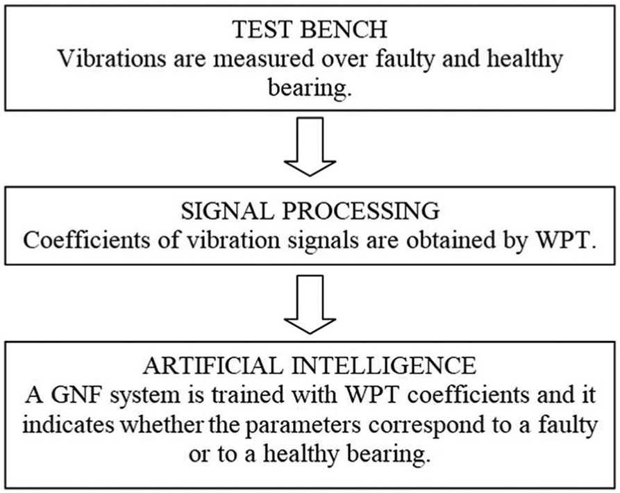
Flowchart of the proposed method.

This article presents a bearing-fault diagnosis technique using an intelligent algorithm. The learning phase intends to process characteristic parameters obtained from WPT which provide information about the internal state of the piece and therefore, to indicate if it is faulty or healthy. This process would determine if the next preventive scheduled maintenance could be extended when the system is healthy or make it scheduled ahead of time if the analyzed piece shows failure indications. In section 1 of this article, a test laboratory bench is presented where different faulty ball bearings are subjected to test and then their vibration signals are measured. In section 2, the methodology to process the signals of each mechanical element is shown. The intelligent technique used to analyze the processed signals in the previous section is presented in section 3. Finally, the results and discussion are shown in section 4.

Experimental data: test bench

The data to test the intelligent system have been obtained from the test lab bench presented in Figure 2. In this bench, developed by the UNED Mechanical Department, FAG 7206 B single ball bearings were tested to prove the suitability of the automated diagnosis method proposed by Castejón et al.²² The test bench has axial and radial pneumatic cylinders for the load, the bearing assembly, a B&K 4383 accelerometer with an 8.5 kHz bandwidth, a photo tachometer device for revolutions per minute (RPM) measurement and a transmission pulley directly connected to a three-phase electric motor by a V-belt. Additional devices are a B&K NEXUS amplifier and a DAS-1200 Keithley acquisition card. The sampling rate was set at 5000 Hz, and each acquired signal had 5120 points.

Figure 2.

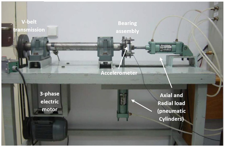
Bearing Test bench: UNED Lab.

Four sets of experiments were performed with the experimental system: under normal conditions (healthy bearings), inner race faults, outer race faults and ball fault. A 2 mm long pit was artificially made in the inner or outer race with an electric pen and multiple slots in the surface were performed to simulate the flacking phenomenon for the rolling ball. Figure 3 shows raw data acquired from all bearing conditions under study.

Figure 3.

Raw data acquired from the test bench from each bearing conditions.

In this point, it is necessary to highlight that the literature and the catalogues of bearing manufacturers consider incipient defects to those whose equivalent surface is between 2 and 5 mm².³⁰

The radial and axial loads were 215 and 200 N, respectively.

For this study, a total of 196 measurements were obtained, 49 for each condition at 600 rpm.

Vibration processing methodology

WPT is especially efficient to locally analyze non-stationary signals.³¹ It obtains correlation coefficients between a signal and a selected mother wavelet function. It consists of the application of the discrete WT in a recursive way until it reaches the selected decomposition level, according to the scheme shown in Figure 4.

Figure 4.

Decomposition tree at level 2 for wavelet packet analysis.

Where W(k, j) represents the coefficients of the signal in each packet, k is the decomposition level and j is the position of the packet within the decomposition level. Then, each correlation vector W(k, j) has the structure of the equation (1)

W (k, j) = {w_{1} (k, j), \dots, w_{n} (k, j), \dots, w_{N} (k, j)}

(1)

where $w_{n} (k, j)$ is the coefficient at position n for the packet.

In order to obtain an efficient number of patterns that describe the dynamic behaviour of the mechanical element to be the input of the intelligent classification system, the energy of each packet has been calculated. The calculation allows reducing considerably the number of inputs by substituting the coefficients of each package by a single value without losing information about the condition of the bearing.

The concept of energy used in wavelet analysis in packages is closely linked to the well-known notions derived from the Fourier Theory. The energy of the wavelet packets is obtained from the sum of the squares of the coefficients of each package according to equation (2)

E_{k, j} = \sum_{n} {| W (k, j) |}^{2}

(2)

In this work, the relative energy of each packet related with the energy of the signal is used as input pattern as equation (3)

e_{k, j} = \frac{E_{k, j}}{\sum_{j} E_{k, j}}

(3)

As an example, in Figure 5, the relative energy corresponding to inner race fault bearing data is shown. The level of decomposition in the example is 3 and the mother wavelet selected is Daubechies 6 (DB6). Owing to the goodness of the results in this area,³² it has been decided to use in this study the level of decomposition 3 and the mother wavelet DB6.

Figure 5.

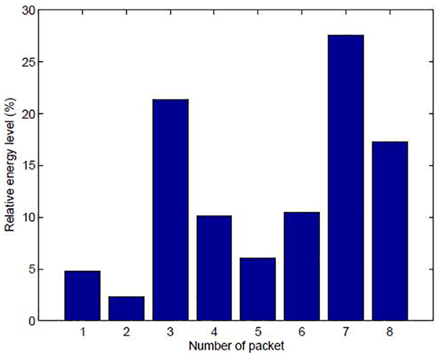
WPT relative energies for inner race fault bearing.

Previous studies with traditional features in time domain and frequency domain such as power spectral density (PSD) or kurtosis were done obtaining good results in severe faults and laboratory conditions,³³ but, if incipient faults have been studied, the amplitude of the spectra is too low to discriminate between signal and noise.

Patterns used to feed the classification system will be the relative energy of each packet. Each packet represents a part of a signal at a specific band frequency. When a fault occurs in a rotatory mechanical element, changes in the energy in certain frequency bands appear. These changes can be clearly presented to the identification system in terms of the energy of the wavelet packet for a better tuning of the condition monitoring system.

Artificial intelligence technique

The main purpose of this work is to build an intelligent system that is able to detect whether the element of the rotary motion drive is faulty or not. Extensive research has been developed in the field of fault diagnosis using several techniques;^{22,28,34–37} however, for this study, a method based on training is the most appropriate one. Particularly, a Neuro-Fuzzy technique^38,39 whose structure is similar to the one proposed by Jang and colleagues^40,41 has been chosen. As it is shown in Figure 6, a three-layer Neuro-Fuzzy is used in which the first layer represents the membership functions, and their inputs are the GNF inputs, whereas their outputs are expressed by equation (4). N₁ being the input number, in this work, N₁ = 8, N₂ is the number of nodes of the intermediate layer, U_i stands for the ith input, m_ij and σ_ij stand for the centre and the width of the membership function, respectively, and, finally, P_ij would be the output neuron with ith input and output connected to jth node of the intermediate layer.

P_{ij} = \exp (\frac{- {(U_{i} - m_{ij})}^{2}}{{σ_{ij}}^{2}}) \begin{matrix} j = 1, 2, \dots, N_{2} \\ i = 1, 2, \dots, N_{1} \end{matrix}

(4)

Figure 6.

Structure of the Neuro-Fuzzy system.

The level 3 discrete wavelet transform (DWT) decomposition applied to the signal provides an eight characteristic coefficient vector, as it was explained in previous sections. This vector will be the input data of the GNF; therefore, the system will have eight inputs.

The rule system is represented by the second layer, whose outputs are obtained by equation (5)

\begin{matrix} λ_{i} = \min | p_{1 j}, p_{2 j}, \dots, p_{N_{1} j} | & j = 1, \dots, N_{2} \end{matrix}

(5)

In the third layer, the defuzzification process is achieved and the global system output is reached by equation (6). N₃ represents the GNF output number; in this work, there are two outputs, and each one is the estimated value of kth output given by jth node

\begin{matrix} Y_{k} = \frac{\sum_{j = 1}^{N_{2}} s v_{jk} λ_{j}}{\sum_{j = 1}^{N_{2}} λ_{j}} & k = 1, \dots, N_{3} \end{matrix}

(6)

As the presented equations show, the described Neuro-Fuzzy system depends on several parameters: the centre (m_ij) and width (σ_ij) of the membership function, the estimated system outputs (sv_jk) and the number of nodes of the intermediate layer (N₂). This set of values will be obtained through a three-phase learning algorithm. The first two phases will provide initial values to several parameters and will optimize the number of nodes of the hidden layer, that is, the number of rules. Finally, the third one resets the parameters obtained in the previous one.

Unsupervised learning phase

The aim of this first phase is to provide initial values to the centre of the membership function (m_ij) and the estimated system outputs (sv_jk). For that, a Kohonen’s self-organizing⁴² feature map algorithm is applied. The initial weight vector of self-organizing map is obtained through the mean between the maximum and minimum of the input given by the user. Its dimension will be the input numbers (N₁) plus output numbers (N₂) as equation (7) shows

W_{j} = (w_{1 j} w_{2 j} w_{3 j} \dots w_{N_{1} + N_{3} j}) j = 1, 2, \dots, N_{2}

(7)

Moreover, the inputs to the self-organizing map are expressed as follows

V = (U_{1} U_{2} \dots U_{N_{1}} Y_{1} Y_{2} \dots Y_{N_{3}})

(8)

where the vector (U₁, U₂,…, U_N₁) corresponds to the input vector to the GNF system, and (Y₁, Y₂,…, Y_N₃) is the desired output vector.

Particularly, in this work, a monodimensional Kohonen self-organizing map is utilized to achieve the winner node that allows to update the weight in equation (9). As it is known, this learning algorithm is a typical unsupervised learning algorithm. Once the winner node is obtained, that is, after the application of the unsupervised learning algorithm has been concluded, an assignment of the centre of the membership functions (m_ij) and the estimated system outputs (sv_jk) will carry out

m_{ij} = w_{ij}; j = 1, 2, \dots, N_{2}; i = 1, 2

(9)

The values for the estimated outputs are chosen using the rest of components of the same vector as

s v_{jk} = w_{N_{1} + k, j}; k = 1, 2; j = 1, 2, \dots, N_{2}

(10)

It is important to highlight that this is an initial assignment of values for these parameters because they will be updated in new phases of the learning algorithm. However, this initial assignment is an important step in order to achieve better results for the algorithm.

The number of nodes in the hidden layer is related with the number of rules; therefore, this one should be optimized previously, hence the necessity of an optimization process in order to obtain a minimum number of rules.

GA phase

In the previous section, each rule related with a node of the intermediate or hidden layer, that is, N₂, was obtained. Moreover, values for m_ij, y ν_jk were fixed. In addition, values for the parameters σ_ij, are necessary; consequently, a GNF system is built. In this phase, the purpose is to determine adequate values for the parameter sv_jk and to achieve a reduced number of nodes on the hidden layer. The GA^43,44 is an algorithm based on the biological paradigm of genetic evolution where it is necessary to specify the content corresponding to an individual from basic information, known as gene. Particularly, in this work, a vector is established as the individual, and the vector components are the genes. Thus, the components of each vector (individual) consist of a representation of the different hidden nodes by a Boolean value and the σ_ij values. That is, each individual is a vector as equation (11) shows

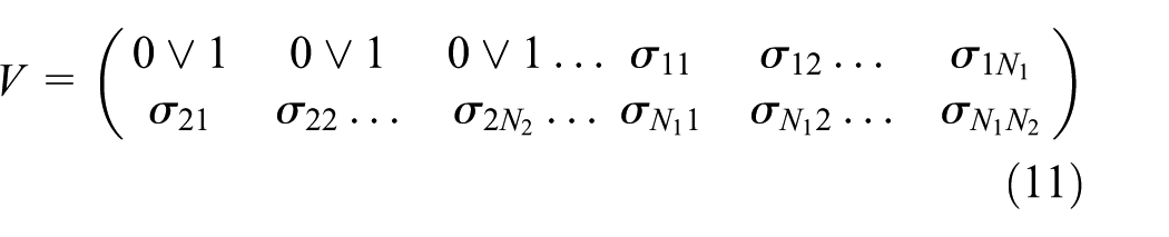
V = (\begin{matrix} 0 \lor 1 & 0 \lor 1 & 0 \lor 1 \dots \\ σ_{21} & σ_{22} \dots & σ_{2 N_{2}} \dots \end{matrix} \begin{matrix} σ_{11} & σ_{12} \dots & σ_{1 N_{1}} \\ σ_{N_{1} 1} & σ_{N_{1} 2} \dots & σ_{N_{1} N_{2}} \end{matrix})

(11)

As it is shown in equation (11), the first N₂ components of vector V are binary values where if there is a 1, it means that this rule is considered in the whole GNF system, whereas if there is a 0 value, it means this rule is eliminated. The last N₁ × N₂ values correspond to the values of σ_ij. The values σ_ij associated to hidden nodes with zero values will not be considered in the implementation of the final result; however, they have been included in equation (8); thus, several individuals are created. Taking into consideration the error between the real output values and the individual output values, a fitness function is defined. Moreover, each individual is a possible trained GNF system and the values obtained in equations (9) and (10) are taken for all individuals in this learning phase. This way, individual satisfactory values for σ_ij and an adequate set of N₂ rules (nodes on the hidden layer) are obtained after the GA is applied.

Supervised learning phase

In this last training phase, the target is to improve the selection of m_ij, σ_ij and sv_jk parameters of the GNF system chosen in previous phases. Owing to the similarity between this system and a neural network built on three layers, the standard learning algorithms adapted to the mathematical expressions of these particular nodes can be applied. The nodes on the input layer have the same mathematical expression as the neurons in a Radial Basis Neural Network.⁴⁵ In fact, the least mean squared learning algorithm could be applied as usual in a typical radial basis network. This algorithm intends to minimize a criterion function. In this case, the error function between the outputs of the GNF system and the real outputs of the available patterns is considered, as equation (12) shows

E = \frac{1}{2} \sum_{k = 1}^{N_{3}} Y_{k} - S_{k}

(12)

where S_k = kth output of the GNF system and Y_k = kth real output.

The initial parameters of the GNF system (m_ij, s_ij, sv_jk and N₂) were fixed in the previous phases of the learning algorithm; thus, this phase only changes these values in order to minimize the error function.

With the data collected in the laboratory, all these phases are applied. The input data are the eight characteristic coefficients of the vector of each measurement, and the output will determine whether the mechanical element is faulty or not. Specifically, this system has two outputs, so that depending on which one is activated, it indicates the case. When the first output is activated (1) and the second one is inactive (0), the signal corresponds to a healthy element; if the first one is inactive (0) and the second one is activated (1), it means that the energy vector comes from an element of rotary motion drive that has a fault.

In each phase, several trials were carried out, so that the parameters that provide an adequate error value were chosen.

Results and discussion

In the laboratory, vibration signals of healthy and faulty mechanical elements were measured and a signal processing was accomplished, particularly a WPT, as it was explained in previous sections. Images of the data used and the first processing corresponding with the spectra PSD can be seen in Castejón et al.²² and the energy of the wavelet packet decomposition can be tested in Gómez et al.⁴⁶ The application of the discrete WT recursively allows for obtaining an adequate number of patterns which describe the dynamic behaviour of the signal. In this study, the level of decomposition is 3 and the mother wavelet selected is DB6; therefore, after this process, there are 1872 data sets, which means 1872 characteristic energy vectors. The data set obtained from the signal processing phase is used in the classification one as input vectors. Particularly, each input vector is composed of eight characteristic coefficients corresponding to each measurement, as it was previously mentioned. The training process was carried out indicating the system if each input vector was coming from a faulty bearing or from a healthy one. In addition, 25% of this set is reserved in order to test the generalization capability of the system; therefore, the training process was carried out with 1404 vectors. Once the training phase is completed, the output will determine whether the mechanical element is faulty or not.

One trial was chosen as it was the one with the best results, that is, the one with minimum error function. As it could be tested in Figures 7 and 8, the error between the estimated output and the provided system output is really small, it is around 10⁻⁵, and even the generalization error is the order of 10⁻⁶. By analyzing the graphs, it can be observed that both error curves seem to continue descending. Nevertheless, after 1000 epochs, the results are satisfactory and the relation between computing time and the error level is adequate. Therefore, even though lower error would be reached, this will not provide quite better results.

Figure 7.

Evolution of quadratic error in training pattern.

Figure 8.

Evolution of quadratic error in test pattern.

In this moment, it is necessary to point out that both outputs are complementary; this means that two values must make 1. This was made in this way due to the characteristics of the system. Given that only one output should be activated, output equal 1, to indicate if the mechanical element is faulty or not, the other one has to be inactive, equal 0. This behaviour is shown in Table 1, where the outputs provided by the system are shown. For this reason, in Figures 7 and 8, only one output is drawn, since similar results were obtained to the other output.

Table 1.

Comparison between output values of the Genetic Neuro-Fuzzy system and desired output.

Input	GNF output	Desired output	State of piece
[0.0118 0.0064 0.0035 0.0024 0.0136 0.0116 0.0066 0.0050]	0.0016 0.9984	0 1	Faulty
[0.0046 0.0047 0.0052 0.0028 0.0059 0.0097 0.0042 0.0063]	−0.0007 1.0007	0 1	Faulty
[0.0020 0.0035 0.0037 0.0026 0.0040 0.0038 0.0041 0.0063]	−0.0010 1.0010	0 1	Faulty
[0.0732 0.0592 0.6486 0.1427 0.0977 0.1343 0.4191 0.2632]	−0.0000 1.0000	0 1	Faulty
[0.0083 0.0150 0.0484 0.0175 0.1877 0.1323 0.0888 0.0790]	1.0003 –0.0003	1 0	Healthy
[0.0099 0.0115 0.0500 0.0182 0.1559 0.0856 0.1061 0.0492]	1.0009 –0.0009	1 0	Healthy
[0.0142 0.0160 0.0684 0.0227 0.1635 0.1567 0.1114 0.0886]	1.0005 –0.0005	1 0	Healthy

Table 1 shows a result comparison. Table 1 presents several examples of response systems over some inputs. It is important to note that in order to check the GNF system, the inputs correspond to those data that were reserved for the test, that is, the shown inputs are unknown to the system. The first four data sets correspond to energy characteristic vector of faulty mechanical elements, whereas the three remaining are of healthy elements. The table allows contrasting the output provided by the GNF system with those that should be. As it can be tested, the trained system reaches a great generalization and it provides the adequate output. Therefore, the GNF system, after being trained, is able to indicate whether an element of rotary motion drive is faulty or not.

Conclusion

In this article, an automatic fault detection technique based on a GNF system has been developed. The DWT decomposition applied over the vibration signal measurements has provided characteristic information about the state of the elements of rotary motion drives. The characteristic vector contains information about whether the mechanical element is faulty or not. Using these vectors as inputs of the GNF has automated the detection process, thus the GNF system could be used for early fault detection at incipient level; therefore, an automatization of the whole maintenance process in real industries could be achieved.

Footnotes

Handling Editor: Xiao-Jun Yang

Declaration of conflicting interests

The author(s) declared no potential conflicts of interest with respect to the research, authorship, and/or publication of this article.

Funding

The author(s) disclosed receipt of the following financial support for the research, authorship, and/or publication of this article: This work was supported by Spanish Government (MAQ-STATUS DPI2015-69325-C2) and (DPI2015-69 1808271602) of Ministerio de Economía y Competitividad and with European Funds of Regional Development (FEDER).

ORCID iD

Angela Hernández

References

Lei

, et al. Fault diagnosis of rotating machinery based on multiple ANFIS combination with GAs. Mech Syst Signal Pr 2007; 21: 2280–2294.

Zhang

, et al. Fault diagnosis of rotating machinery based on improved wavelet package transform and SVMs ensemble. Mech Syst Signal Pr 2007; 21: 688–705.

Lou

Loparo

KA.

Bearing fault diagnosis based on wavelet transform and fuzzy inference. Mech Syst Signal Pr 2004; 18: 1077–1095.

Gomez

Castejon

Garcia-Prada

. Incipient fault detection in bearings through the use of WPT energy and neural networks. In: Dalpiaz

Rubini

D’Elia

, et al. (eds) Advances in condition monitoring of machinery in non-stationary operations. Berlin, Heidelberg: Springer, 2014, pp.63–72.

Huang

Ouyang

Gao

, et al. A feature extraction method for vibration signal of bearing incipient degradation. Meas Sci Rev 2016; 16: 149–159.

Caesarendra

Tjahjowidodo

Kosasih

, et al. Integrated condition monitoring and prognosis method for incipient defect detection and remaining life prediction of low speed slew bearings. Machines 2017; 5: 11.

Zhou

Duan

Mba

, et al. A comparative study of helicopter planetary bearing diagnosis with vibration and acoustic emission data. In: Proceedings of the 2017 IEEE international conference on prognostics and health management (ICPHM), Dallas, TX, 19–21 June 2017, pp.246–251. New York: IEEE.

Costa Castelló

Puig

Blesa

. Introducción a la Diagnosis de Fallos basada en Modelos mediante Aprendizaje basado en Proyectos. Rev Iberoam Automática E Informática Ind RIAI 2016; 13: 186–195.

Abé

Igusa

Semi-active dynamic vibration absorbers for controlling transient response. J Sound Vib 1996; 198: 547–569.

10.

Blanco-Ortega

Beltrán-Carbajal

Silva-Navarro

, et al. Control de Vibraciones en Maquinaria Rotatoria. Rev Iberoam Automática E Informática Ind RIAI 2010; 7: 36–43.

11.

Beltrán-Carbajal

Silva-Navarro

Arias-Montiel

Control Activo de Vibraciones en un Rotor Tipo Jeffcott con Velocidad Variable Usando una Suspensión Electromecánica. Rev Iberoam Automática E Informática Ind RIAI 2014; 11: 295–303.

12.

Yang

Application of the EMD method in the vibration analysis of ball bearings. Mech Syst Signal Pr 2007; 21: 2634–2644.

13.

Rai

Mohanty

AR.

Bearing fault diagnosis using FFT of intrinsic mode functions in Hilbert–Huang transform. Mech Syst Signal Pr 2007; 21: 2607–2615.

14.

Wang

Luo

Qin

, et al. Fault identification and classification of rolling element bearing based on time-varying autoregressive spectrum. Mech Syst Signal Pr 2008; 22: 934–947.

15.

Tao

Zhu

Ding

, et al. An alternative time-domain index for condition monitoring of rolling element bearings – a comparison study. Reliab Eng Syst Saf 2007; 92: 660–670.

16.

Mallat

A wavelet tour of signal processing. New York: Academic Press, 2007, pp.83–85.

17.

Wang

McFadden

. Application of the wavelet transform to gearbox vibration analysis. In: Proceedings of the 16th annual energy sources technology conference and exposition, Houston, TX, 31 January–4 February 1993, pp.13–20. New York: American Society of Mechanical Engineers (ASME).

18.

Adewusi

Al-Bedoor

BO.

Wavelet analysis of vibration signals of an overhang rotor with a propagating transverse crack. J Sound Vib 2001; 246: 777–793.

19.

Baydar

Ball

Detection of gear failures via vibration and acoustic signals using wavelet transform. Mech Syst Signal Pr 2003; 17: 787–804.

20.

Xiang

Zhong

Chen

, et al. Crack detection in a shaft by combination of wavelet-based elements and genetic algorithm. Int J Solids Struct 2008; 45: 4782–4795.

21.

Douka

Loutridis

Trochidis

Crack identification in beams using wavelet analysis. Int J Solids Struct 2003; 40: 3557–3569.

22.

Castejón

Lara

García-Prada

JC.

Automated diagnosis of rolling bearings using MRA and neural networks. Mech Syst Signal Pr 2010; 24: 289–299.

23.

Liu

Ling

S-F

Meng

QF.

Machinery diagnosis based on wavelet packets. J Vib Control 1997; 3: 5–17.

24.

Shen

Wang

Kong

, et al. Fault diagnosis of rotating machinery based on the statistical parameters of wavelet packet paving and a generic support vector regressive classifier. Measurement 2013; 46: 1551–1564.

25.

Feng

Schlindwein

FS.

Normalized wavelet packets quantifiers for condition monitoring. Mech Syst Signal Pr 2009; 23: 712–723.

26.

Chow

M-Y

Sharpe

Hung

. On the application and design of artificial neural networks for motor fault detection. II. IEEE T Ind Electron 1993; 40: 189–196.

27.

Lara Castro

Sisamón

Garcia Prada

JC.

Bearing fault diagnosis based on neural network classification and wavelet transform. In: Proceedings of the 6th WSEAS international conference on wavelet analysis & multirate systems, Bucharest, 16–18 October 2006, pp.22–29. New York: ACM.

28.

Ben Ali

Fnaiech

Saidi

, et al. Application of empirical mode decomposition and artificial neural network for automatic bearing fault diagnosis based on vibration signals. Appl Acoust 2015; 89: 16–27.

29.

Staszewski

. Vibration data compression with optimal wavelet coefficients. In: Proceedings of the second international conference on genetic algorithms in engineering systems: innovations and applications, Glasgow, 2–4 September 1997, pp.186–190. New York: IEEE.

30.

Tra

Kim

Khan

, et al. Incipient fault diagnosis in bearings under variable speed conditions using multiresolution analysis and a weighted committee machine. J Acoust Soc Am 2017; 142: EL35–EL41.

31.

Gómez

Castejón

García-Prada

, et al. Review of recent advances in the application of the wavelet transform to diagnose cracked rotors. Algorithms 2016; 9: 19.

32.

Castejón

García-Prada

Gómez

, et al. Automatic detection of cracked rotors combining multiresolution analysis and artificial neural networks. J Vib Control 2015; 21: 3047–3060.

33.

Sánchez

R-V

Lucero

Vásquez

, et al. Feature ranking for multi-fault diagnosis of rotating machinery by using random forest and KNN. J Intell Fuzzy Syst 2018; 34: 3463–3473.

34.

Bordoloi

Tiwari

Support vector machine based optimization of multi-fault classification of gears with evolutionary algorithms from time-frequency vibration data. Measurement 2014; 55: 1–14.

35.

Korbicz

Fault diagnosis: models, artificial intelligence, applications. Berlin; Heidelberg, Springer, 2004, p.920.

36.

Siddique

Yadava

Singh

. Applications of artificial intelligence techniques for induction machine stator fault diagnostics – review. In: Proceedings of the 4th IEEE international symposium on diagnostics for electric machines, power electronics and drives, 2003 (SDEMPED 2003), Atlanta, GA, 24–26 August 2003. pp.29–34. New York: IEEE.

37.

Tallam

Habetler

Harley

RG.

Self-commissioning training algorithms for neural networks with applications to electric machine fault diagnostics. IEEE T Power Electron 2002; 17: 1089–1095.

38.

Mitra

Hayashi

Neuro-fuzzy rule generation: survey in soft computing framework. IEEE T Neural Networ 2000; 11: 748–768.

39.

Marichal

Hernández

Acosta

, et al. A Neuro-Fuzzy system for extracting environment features based on ultrasonic sensors. Sensors 2009; 9: 10023–10043.

40.

Jang

JSR

. ANFIS: adaptive-network-based fuzzy inference system. IEEE T Syst Man Cyb 1993; 23: 665–685.

41.

Marichal

Artés

García Prada

, et al. Extraction of rules for faulty bearing classification by a Neuro-Fuzzy approach. Mech Syst Signal Pr 2011; 25: 2073–2082.

42.

Kohonen

The self-organizing map. Proc IEEE 1990; 78: 1464–1480.

43.

Samanta

Al-Balushi

Al-Araimi

SA.

Bearing fault detection using artificial neural networks and genetic algorithm. EURASIP J Adv Sig Pr 2004; 2004: 366–377.

44.

Goldberg

Holland

JH.

Genetic algorithms and machine learning. Mach Learn 1988; 3: 95–99.

45.

Chen

Cowan

CFN

Grant

PM.

Orthogonal least squares learning algorithm for radial basis function networks. IEEE T Neural Networ 1991; 2: 302–309.

46.

Gómez

Castejón

Corral

, et al. Analysis of the influence of crack location for diagnosis in rotating shafts based on 3 x energy. Mech Mach Theory 2016; 103: 167–173.

Wavelet Packets Transform processing and Genetic Neuro-Fuzzy classification to detect faulty bearings

Abstract

Keywords

Introduction

Experimental data: test bench

Vibration processing methodology

Artificial intelligence technique

Unsupervised learning phase

GA phase

Supervised learning phase

Results and discussion

Conclusion

Footnotes

Declaration of conflicting interests

Funding

ORCID iD

References