Sage Journals: Discover world-class research

Abstract

The plasticity models in finite element codes are often not able to describe the cyclic plasticity phenomena satisfactorily. Developing a user-defined material model is a demanding process, challenging especially for industry. Open-source Code_Aster is a rapidly expanding and evolving software, capable of overcoming the above-mentioned problem with material model implementation. In this article, Chaboche-type material model with kinematic hardening evolution rules and non-proportional as well as strain memory effects was studied through the calibration of the aluminium alloy 2024-T351. The sensitivity analysis was performed prior to the model calibration to find out whether all the material model parameters were important. The utilization of built-in routines allows the calibration of material constants without the necessity to write the optimization scripts, which is time consuming. Obtaining the parameters using the built-in routines is therefore easier and allows using the advanced modelling for practical use. Three sets of material model parameters were obtained using the built-in routines and results were compared to experiments. Quality of the calibration was highlighted and drawbacks were described. Usage of material model implemented in Code_Aster provided good simulations in a relatively simple way through the use of an advanced cyclic plasticity model via built-in auxiliary functions.

Keywords

Chaboche kinematic hardening Armstrong–Frederick model Voce isotropic hardening biaxial stress ratcheting multiaxial fatigue

Introduction

Material points in the structure undergo various types of loadings. The monotonic loading occurs mostly in the manufacturing processes or accidents, but it is rather exceptional when compared to the repeated (cyclic) one, which can be regarded as the most frequent in operating conditions. It is crucial to be aware of the loading nature, especially in the cases where the hazard to human safety is imminent. Examples of structures with such scenarios include transportation (automotive, aircraft, marine or railway), power production (hydro or nuclear) and many others.

The cyclic loading is often not just uniaxial, which has been covered very well in the literature,^1,2 but multiaxial and, moreover, non-proportional.³ The commercial software such as ANSYS or Abaqus supports some advanced plasticity models with limited potential for customization. There is definitely an option for implementing a user material definition to the commercial codes, but this is still rather expensive and time-consuming. The alternative way is to use an open-source programme such as Code_Aster developed by EDF’s R&D, which provides the possibility of using the advanced models of cyclic plasticity.⁴ It is distributed as a free software under the terms of the GNU General Public Licence, so users can easily contribute to the programme development. The code has its limitations, but it has been rapidly developed in the recent years. The user base has been growing, which has been accompanied along with a better support across the community. The software offers a solution to the problems of solid mechanics, thermomechanics and associated phenomena with a support of C and Python programming languages. The service developed by EDF is used, for example, by Bureau Veritas, French Alternative Energies, Atomic Energy Commission or PRINCIPIA.⁵

In the area of cyclic plasticity, Chaboche et al.⁶ presented a basic non-linear combined hardening law-based constitutive model. It is composed of the superimposed kinematic hardening rules proposed by Armstrong and Frederick⁷ and Voce⁸ based on isotropic hardening model, which was improved in order to account for the strain memory effect. Burlet and Cailletaud⁹ modified the dynamic recovery term to become the radial evanescence term in the model proposed by Armstrong and Frederick.⁷ Chaboche¹⁰ later proposed the modification of the kinematic hardening in order to improve the ratcheting behaviour. Bari and Hassan¹¹ introduced a new parameter in order to obtain better results in the ratcheting simulations of multiaxial loading. A parameter accounting for the non-proportionality was introduced by Benallal and Marquis.¹² It was incorporated into the isotropic hardening. Tanaka¹³ introduced the fourth-order tensor, which described the slow growth of the internal dislocation structure induced by the plastic deformation, which served as the definition of another non-proportionality parameter. Hassan et al.¹⁴ proposed to incorporate the influence of non-proportional loading on the ratcheting responses through the kinematic hardening-related parameters. Krishna et al.¹⁵ suggested introducing the dependence of the kinematic hardening and multiaxial parameter on the hardening variable – the plastic strain surface – when the material is dependent on the loading amplitude and does not exhibit the behaviour described by Masing.¹⁶

The isotropic hardening was modified in order to incorporate the influence of non-proportionality as well as softening, which allows starting with the monotonic yield surface and subsequently reduce its size quickly. This is necessary because the yield stress under the monotonic loading is usually larger than that under the cyclic one. Then, the yield surface size and curve shape evolution from monotonic to the first reversal can be accommodated. Finally, the model should be calibrated using three amplitudes at least. First, it is the amplitude where the cyclic stress–strain curve starts to deviate from the monotonic one, next the amplitude where the two curves become equidistant and last, some amplitude (or more) between the latter two.

Khutia el al.¹⁷ presented the dependency of kinematic hardening parameters on the plastic strain surface within the model proposed by Ohno and Wang,^18,19 which presents another alternative to the approach developed by Chaboche et al.⁶ Abdel-Karim²⁰ modified the model proposed by Ohno and Wang^18,19 by introducing the radial evanescence term into the model as presented by Burlet and Cailletaud⁹ earlier. Another modification to the model was made by Abdel-Karim²¹ in order to incorporate the isotropic hardening associated with the kinematic one in the constitutive equations, where the activation of respective hardening was governed by a specific parameter. Meggiolaro et al.²² introduced new integral estimates for the non-proportionality factor of periodic loadings using the concept of Tanaka.¹³ Later, Meggiolaro et al.^23,24 presented a unified approach to the modelling of non-linear kinematic hardening represented in the five-dimensional space for applications to the mean stress relaxation and multiaxial ratcheting, which can also reproduce the multi-surface approach proposed by Mróz,²⁵ where the plastic modulus calculation is not coupled to the kinematic hardening rule through the consistency condition as in the previous cases, but it still might be indirectly influenced. Hence, the so-called uncoupled model.

The number of material constants increases with the complexity of the model, which can provide a versatile and flexible tool. However, this can lead to enormous number of parameters with unclear physical interpretation, which is rather a mathematical exercise of fitting. Therefore, the sensitivity analysis is important for the minimization of the number of parameters, which are used in the subsequent optimization task. In the end, more robust analysis can be conducted. So, the main goal is to address the experts and designers from the mechanical engineering field to carry out the analyses using the advanced constitutive models, which provide enhancements in the reliability and safety of the structures.

Experiments

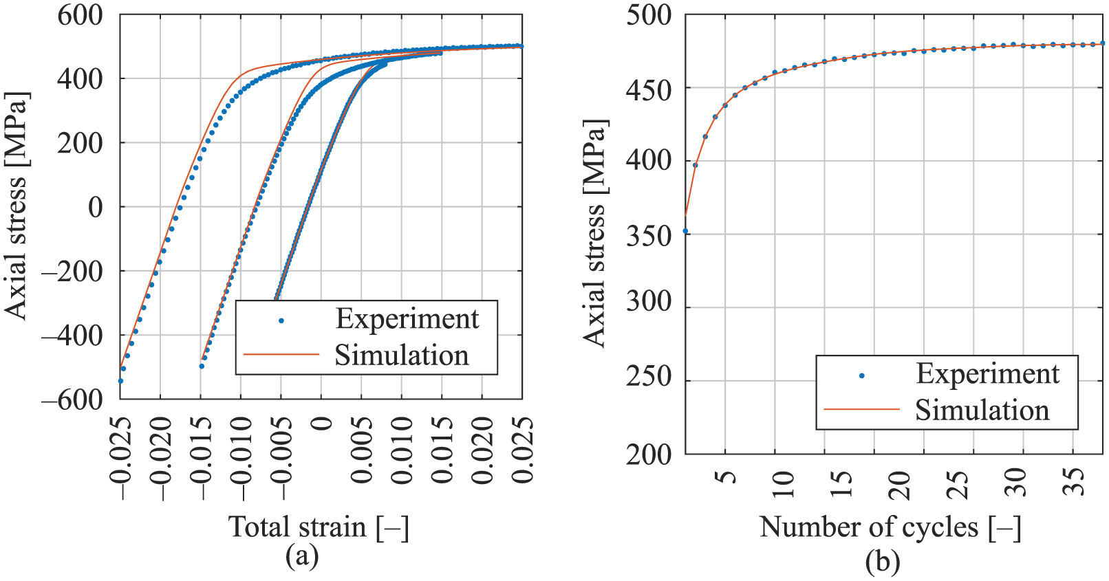
The whole experimental programme was conducted on the aluminium alloy 2024-T351. Experiments and results were taken from the study of Peč et al.²⁶ Here, only the crucial ones needed for the model parameter calibration are summarized. The examined alloy does not exhibit the behaviour according to Masing.¹⁶ The strain-controlled testing on three different amplitude levels was conducted on cylindrical specimens (Figure 1(f)). The first, mid-life (half number of cycles to failure) and last hysteresis loops before failure are depicted in Figure 1(a) for the experiment with 0.8% total strain amplitude for better clarity. Figure 1(b) and (c) represent the loading histories for the strain-controlled testing under 1.5% and 2.5% total strain amplitudes, respectively. These responses were developed to obtain an idea of the effect of loading amplitude and cycle number on the shape of hysteresis loop. The stress-controlled testing was performed with 410 MPa stress amplitude and 20 MPa mean stress. The same specimen as in the case of strain-controlled loading was used (Figure 1(f)). The first, mid-life and last loops before the failure are depicted in Figure 1(d) to show clearly the phenomenon of ratcheting and corresponding hysteresis loop evolution. The three-step experiment was carried out to map the non-proportionality under the strain-controlled regime of 0.7% total strain amplitude (Figure 1(e)). The tubular specimen (Figure 1(g)) was axially loaded in the first and third steps. The second step consisted of the circular loading path in the normal and shear strain space.¹³

Figure 1.

Experiment: (a) strain-controlled test with 0.8% total strain amplitude; (b) strain-controlled test with 1.5% total strain amplitude; (c) strain-controlled test with 2.5% total strain amplitude; (d) stress-controlled ratcheting test with 410 MPa stress amplitude and 20 MPa mean stress; (e) three-step (tension, tension-torsion, tension) non-proportional experiment under 0.7% total strain amplitude; (f) cylindrical specimen; and (g) tubular specimen (dimensions in mm).

Modelling methods

Finite element analysis

The simulations were carried out by means of the finite element method using the freely available software Code_Aster.⁴ Internally implemented macro SIMU_POINT_MAT simulates the mechanical behaviour of one element or just one integration point in the quasi-static loading conditions. All material models with non-linear behaviour are implemented and ready to use. The reason why to use this macro to the simulation of a point response instead of the whole material sample (whole testing specimen) is the simplicity and efficiency (algorithm speed). The user can calculate and evaluate by this macro all the tensor variables presented in the selected model depending on time. No geometry or mesh is needed. This is why the boundary conditions are limited to the strain, stress and gradient tensors. User can specify the individual tensor elements in time to simulate responses under a loading history. All other options are the same as for the standard analysis. Stresses and strains are stored in a table along with all the model internal variables as a function of time.

The loading conditions were replicated from experiments, where the total axial strain or stress was used as a function of time. These conditions allowed us to precisely simulate the loading history and required results could be easily extracted by specifying the desired timestamps.

The material was modelled using the operator DEFI_MATERIALU, which has a composition depending on the desired behaviour. The aluminium alloy 2024-T351 was modelled as a combination of the constant linear elastic characteristics given by a keyword ELAS and the constant non-linear characteristics described by keywords CIN2_CHAB (combination of the two non-linear evolution rules proposed by Armstrong and Frederick⁷), CIN2_NRAD (contribution of the non-proportionality effects) and MEMO_ECRO (association of some parameters with the strain memory effect depending on the work hardening).

The rate-independent elastic–plastic material model implemented in Code_Aster⁴ includes the associated flow rule, small strain theory and isothermal conditions. The additive law for the total strain is defined as a sum of elastic and plastic strains, $ε^{e}$ and $ε^{p}$ , respectively, by

d \underline{ε} = d {\underline{ε}}^{e} + d {\underline{ε}}^{p}

(1)

where underline denotes the tensor quantity. Hooke’s law describes the linear elasticity for stress as

d \underline{σ} = \underline{\underline{D}} : d {\underline{ε}}^{e}

(2)

where $\underline{\underline{D}}$ is the fourth-order elasticity tensor and ‘:’ denotes the tensor product.

The yield function is formulated as

f (\underline{s} - \underline{a}) = J (\underline{s} - \underline{a}) - Y

(3)

where $\underline{s}$ is the deviatoric stress tensor, $\underline{a}$ is the deviatoric backstress tensor, Y is the yield stress and $J (\underline{s} - \underline{a})$ is von Mises stress invariant defined as

J (\underline{s} - \underline{a}) = \sqrt{\frac{3}{2} (\underline{s} - \underline{a}) : (\underline{s} - \underline{a})}

(4)

The incremental plastic strain tensor (numerical form of an associated flow rule) is written as

d {\underline{ε}}^{p} = \frac{3}{2} \frac{\underline{s} - \underline{a}}{J (\underline{s} - \underline{a})} d p

(5)

where $d p$ is the magnitude of the plastic strain increment.

The yield stress evolution is given by the expression including the initial yield stress $σ^{y 0}$ and the isotropic hardening R as

Y = σ^{y 0} + R

(6)

The isotropic hardening evolution is then formulated as

d R = b (Q - R) d p

(7)

and

Q = Q^{0} + (Q^{\infty} - Q^{0}) (1 - e^{- 2 μ q})

(8)

where b is the stabilization rate of R, Q is the saturated value of isotropic hardening dependent on the maximum plastic strain, $Q^{0}$ is the initial value of Q, $Q^{\infty}$ is the saturated value of Q, $μ$ is the stabilization rate of Q and q is the radius of the surface in the plastic strain space equivalent to Y in the stress space.

The strain memory effect is included in order to account for the strain range dependency as

g ({\underline{ε}}^{p} - \underline{ξ}) = \frac{2}{3} J ({\underline{ε}}^{p} - \underline{ξ}) - q

(9)

where $g ({\underline{ε}}^{p} - \underline{ξ})$ and $J ({\underline{ε}}^{p} - \underline{ξ})$ are the equivalents to the yield function $f (\underline{s} - \underline{a})$ and von Mises stress invariant $J (\underline{s} - \underline{a})$ . The internal variable $\underline{ξ}$ is equivalent to $\underline{a}$ in the stress space, and it is defined within the strain space as

d \underline{ξ} = (1 - η) \frac{d q}{η} {\underline{n}}^{*}

(10)

where $η$ is the user-defined parameter to control the level of strain memory effect present in the model. This parameter can also be seen as a parameter defining whether there is a kinematic or isotropic shift of the strain memory surface in the space of plastic strains. The evolution of the plastic strain surface is written as

d q = η H (g) < \underline{n} : {\underline{n}}^{*} > d p

(11)

where $H (\dots)$ is the Heaviside step function, <…> denotes Macaulay’s brackets, $\underline{n}$ is the unit normal to the yield surface and ${\underline{n}}^{*}$ is the unit normal to the strain memory surface, which reads

{\underline{n}}^{*} = \frac{3}{2} \frac{{\underline{ε}}^{p} - \underline{ξ}}{J ({\underline{ε}}^{p} - \underline{ξ})}

(12)

The kinematic hardening consists of the two superimposed non-linear evolution rules proposed by Armstrong and Frederick⁷

d \underline{a} = \sum_{i = 1}^{2} d {\underline{a}}_{i}

(13)

where i is the number of particular evolution rule

d {\underline{a}}_{i} = \frac{2}{3} C_{i} d {\underline{ε}}^{p} - γ_{i} (δ_{i} {\underline{α}}_{i} + (1 - δ_{i}) ({\underline{α}}_{i} : \underline{n}) \underline{n}) d p

(14)

where C and $γ$ are the parameters related to the shape of loops and $δ$ is the non-proportionality parameter. Kinematic hardening parameters can be dependent on the accumulated plastic strain as (or otherwise according to Chaboche²⁷)

C_{i} = C_{i}^{\infty} (1 + (k - 1) e^{- wp})

(15)

where $C^{\infty}$ is the saturated value of C, k is the parameter influencing the level of C evolution (C is a constant when $k = 1$ ), w is the stabilization rate of C and

γ_{i} = γ_{i}^{0} (a^{\infty} + (1 - a^{\infty}) e^{- bp})

(16)

where $γ^{0}$ is the initial value of $γ$ and $a^{\infty}$ is the material constant.

A specific functionality of each parameter is summarized in Table 1 together with particular necessary experiment for the parameter determination.

Table 1.

Functionality of specific parameters.

Parameter	Functionality	Meaning	Required experiment/cycle
E, $ν$	Linear elastic	Defines Hooke’s law by $\underline{\underline{D}}$	Monotonic tensile test
b	Cyclic hardening	Rate of isotropic hardening evolution (generally) and the kinematic hardening by modifying $γ_{i}$ in the hereinafter used model	Peak stresses from each cycle of the strain-controlled test
$C_{1}^{\infty}$ , $C_{2}^{\infty}$	Cyclic hardening	Shape of loops in the sense of tangent	Saturated hysteresis loop from the strain-controlled test with a reasonable loading amplitude (so that the upper branch is almost horizontal)
$η$	Cyclic hardening	Rate of kinematic hardening evolution	First few cycles (about 20) from the strain-controlled test
$γ_{1}^{0}$ , $γ_{2}^{0}$	Cyclic hardening and ratcheting	Shape of loops in the sense of slope	First cycle of the strain-controlled test with a reasonable loading amplitude
$μ$ , $Q^{0}$ , $Q^{\infty}$	Cyclic hardening	Size of the isotropic hardening due to the various loading amplitudes	Multiple dependencies of the maximum stress on the number of cycles from the strain-controlled test
$σ^{y 0}$	Plasticity	Defines an elastic region	First cycle of the strain-controlled test
$δ_{i}$	Non-proportionality	Defines a model response to the multiaxial loading	Out-of-phase non-proportional loading test
k,w, $a^{\infty}$	Evolution of parameters	Defines the evolution of other parameters	–

Sensitivity analysis

Most models for simulations are complex with many parameters, state variables and non-linear relations. Those models have many degrees of freedom and are able to produce almost any desired result with some effort.²⁸ This is the reason of cynical opinion about the models.²⁹ The importance of the input parameters with respect to the model output needs to be quantified for this reason. Global, quantitative and model-free (independent of model assumptions) sensitivity analysis needs to be performed to evaluate the robustness and parameter’s importance. Moreover, it was noted that the theoretical methods are sufficiently advanced, so that it is intellectually dishonest to perform the modelling without the sensitivity analysis.³⁰

MATLAB Statistics and Machine Learning Toolbox supports variety of methods to define the parameter importance such as the correlation and partial correlation in various forms. Pearson’s correlation coefficient is a linearity measure between the parameter and the output. It takes value from −1 to 1, where −1 and 1 mean the linear relationship (indirect and direct correlation, respectively) and 0 means no dependency. Partial correlation coefficient is similar to the previous one with an exception that effects of other parameters are cancelled.³¹

Python SALib (Sensitivity Analysis Library) package is an open-source library for the sensitivity analysis with the methods of Sobol’, Morris and others. The sensitivity of each input is represented by a numeric value for the Sobol’ sensitivity analysis, which is called the sensitivity index. It comes in several forms:

The first-order index S1 measures the output variance caused by a single parameter. Higher value means higher dependence of output on a certain parameter.

The second-order index S2 measures the output variance caused by the interaction of two parameters. Strong interactions between the parameters can be found if indices are subtracted from each other.

The total-order index ST is the sum of all previous indices. There is a possibility of higher-order index interactions if the total-order indices are much larger than the first-order one.³²

The method of Morris allows classifying the inputs into three groups: inputs having negligible effects, inputs having large linear effects without interactions and inputs having large non-linear and/or interaction effects:^31,33

$μ^{*}$ measures the influence of the parameter on output. Higher value means higher dependence of output on a certain parameter.

$σ^{*}$ is the measure of the non-linear and/or interaction effects of the parameter on the output. Small values mean linear relationships and large values mean non-linear effects or interactions with other parameters.^31,34

Determination of parameters

MACR_RECAL macro forms a relationship between the Code_Aster simulation results from SIMU_POINT_MAT (and others of course) and experimental (user-defined) data. The macro was used to determine the material model parameters to describe the experimental data sufficiently in this case.

The user has to define N number of experimental curves (tensile branches from loops), P number of parameters with defined ranges and initial values and N number of simulated curves (in tables). Experimental data and optimization settings with definitions of parameters are defined in the master file and simulations are executed in the slave file, which is called by the master file as shown in Figure 2. It is an iterative process, where the master file creates parameters based on the previous results.

Figure 2.

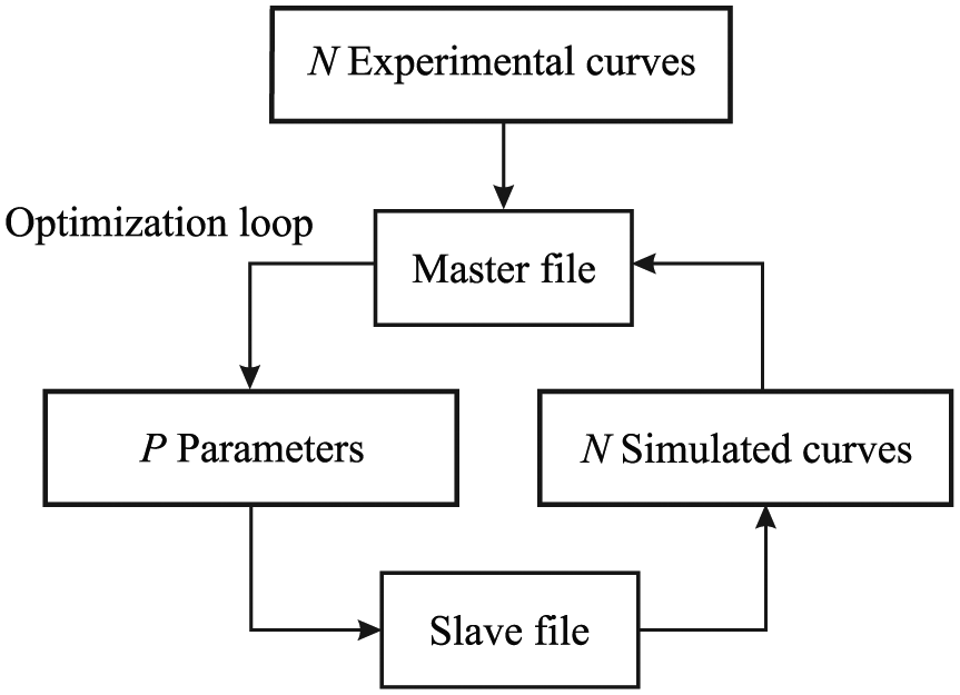
General MARC_RECAL flow chart.⁴

The initial guess of parameters was done by a standard technique described in many works.^6,15 It consisted of approximate identification of $C_{i}^{\infty}$ , $γ_{i}^{0}$ and $σ^{y 0}$ from the first and saturated loops of experiment under 2.50% total strain amplitude.

Different optimization techniques can be chosen in optimization settings such as Levenberg–Marquardt algorithm, genetic, hybrid and others. Levenberg–Marquardt algorithm is based on the gradients and because of that, it is not suitable for finding a global minimum for highly non-linear models. The genetic algorithm stands for the evolutionary algorithms and the hybrid one is a combination of Levenberg–Marquardt and genetic algorithms, where the parameter space is searched roughly by a genetic algorithm and then analysed by a gradient method.

Evolutionary algorithms are the special type of computing method inspired by the process of natural evolution. The main idea of all evolutionary algorithms is the same: environmental pressure is applied to a given population causing a rise of the population fitness. Based on the fitness, suitable candidates are chosen to seed the next generation by applying the recombination and/or mutation to them. This leads to a set of new candidates (the offspring), which competes based on their fitness with the old ones for a place in the next generation. This process of creating new generations and selecting the candidates is the iterative process until a feasible and sufficient solution is found or some limit is reached. The general schema of evolutionary algorithm is show in Figure 3.

Figure 3.

Evolutionary algorithm flow chart.³⁵

Results and discussions

Two different simulations were done in order to obtain the final results and give a good perspective on the issues raised. The first simulation excluded the stress-controlled loading from the optimization process, while the second one included it. The separate stress-controlled loading simulation was performed and no convergence was obtained after finishing the first simulation, which excluded the stress-controlled loading alone. The process of model calibration was carried out in three steps. First, separated simulations with a full model were fine-tuned and exceptions were created to prevent the failure of the file execution. Second, the design points of all the model parameters were created and simulated using the routine from the first step and the sensitivity analysis was performed. And finally, important parameters (all parameters in the end – see the following subsections) were selected according to the sensitivity analysis and the model calibration was completed.

The weighted sum of squared residuals was used to obtain the single quantity since the multiple simulations were carried out under different loading conditions and only a single objective optimization was available. The strain loading was weighted by the following values: $w_{j} = [0.1, 0.3, 0.1, 1.0]$ , where the first three values stand for the tensile branches of saturated loops and the fourth one is for the maximum tensile stress peaks over each cycle. The greatest emphasis was placed on the stress evolution (the last value, 1.0) since it is the most important because the shape of loops cannot be described well with the only two kinematic hardening rules. The shape of the loops was calibrated to best capture the loading with the total strain amplitude of 1.50% (the second value, 0.3). The formula for classical least-squares method was

S = \sum_{i = 1}^{n} {(σ_{i}^{\exp} - σ_{i}^{sim})}^{2}

(17)

where n is the number of either division of tensile branches or tensile stress peaks, and $σ^{\exp}$ and $σ^{sim}$ are the stresses from experiment and simulation, respectively. Then, the weighted sum of squared residuals was

WS = \sum_{j = 1}^{4} w_{j} S_{j}

(18)

Sensitivity analysis results

This subsection shows the results of sensitivity analysis under two conditions. The sensitivity was evaluated separately under the strain- and stress-controlled loading in order to separate the effects of individual parameters. However, it is important to have an idea of overall model behaviour. Particular attention must be paid to all parameters and their meaning must be clearly known. Their importance will be discussed later after the evaluation of the stress-controlled loading sensitivity.

Strain-controlled tests

Methods of Sobol’ and Morris showed that all parameters had influence on outputs, but Pearson’s and partial correlation methods revealed no influence of $η$ , k and w parameters on outputs. Both methods gave almost identical results and suggested that $η$ , k and w parameters can be neglected in the case of strain-controlled loading (Figure 4). Their significance has to be re-evaluated later, because the parameter evolution is needed.

Figure 4.

Pearson’s and partial correlation coefficients for the strain-controlled loading.

The evaluation of S1 index showed that the output was almost identically dependent on the variance of single parameter (Figure 5). However, it showed high level of non-linearity and/or parameter interactions since ST and S1 difference was high.

Figure 5.

Sobol’ sensitivity coefficients for the strain-controlled loading.

Morris method showed that all parameters were important for the model simulation as it can be seen in Figure 6.

Figure 6.

Morris coefficients for the strain-controlled loading.

Stress-controlled tests

Sobol’ method showed that all parameters had influence on outputs, but Pearson’s and partial correlation methods showed almost zero influence of $a^{\infty}$ and $C_{1}^{\infty}$ parameters on outputs (Figure 7).

Figure 7.

Stress-controlled loading: (a) Pearson’s and partial correlation coefficients; (b) Sobol’ sensitivity coefficients.

Influence of parameters $η$ , $a^{\infty}$ , k and w was tied together since all of them somehow represent the evolution of parameters and the associated stress evolution: $η$ gives the evolution of isotropic hardening; and $a^{\infty}$ , k and w give the evolution of kinematic hardening ( $a^{\infty}$ particularly for the evolution of $γ$ and k with w for the evolution of C). One of these four parameters is essential for the different sensitivity analysis because the calibration of the mentioned model is highly non-linear, which can be seen from the equations themselves and Sobol’ results. The calibration might be stable if one set of parameters for isotropic as well as for kinematic hardening is used, but different set of parameters is dominant for different loading conditions. All of them were used for calibration for this reason. Another reason might be that many authors have used much more complicated models with greater number of parameters.^36–39

Multiaxial tests

Last parameters associated with the multiaxial loading are $δ_{1}$ and $δ_{2}$ . The sensitivity can be evaluated by a visual inspection since there are just two parameters to be determined. This is also possible because all other parameters were fixed with the values defined in the last column of Table 1. The error is plotted and coloured according to its value for each pair of parameters generated by the Latin Hypercube Sampling (LHS)⁴⁰ method in Figure 8. The LHS was used because it remembers what was already generated and avoids duplicity or generating almost identical points. In total, 100 pairs were generated and evaluated, of which 4 experienced convergence problems (marked by a black cross), while the set of parameters with the smallest error is marked by a red circle in Figure 8. It is clear that $δ_{2}$ has a minimum influence on the error in this case because the error values are almost identical in the vertical direction (have similar colour in Figure 8).

Figure 8.

Graphical evaluation of sensitivity for multiaxial loading.

Finite element analysis results

The elastic constants were represented by Young’s modulus of 72,500 MPa with Poisson’s ratio of 0.34.²⁶

One great advantage of the presented model is its independent calibration for the uniaxial and multiaxial loadings. The uniaxial loading was calibrated until the results were satisfactory in the first step and then only multiaxial parameters ( $δ_{i}$ ) were found in the separate calibration.

Uniaxial loading

Many simulations were run, from which the three best simulations are presented.

The following weighting functions were used in the case of first parameter set (Table 2):

Weights of 0.1, 0.3 and 0.1 were used for the tensile branches of hysteresis loops of 0.8%, 1.5% and 2.5% total strain amplitudes, respectively. The weight values were estimated by the trial-and-error method. Therefore, many simulations were demanded.

Weight of 1.0 was used for the peak stress evolution in each cycle for the total strain amplitude of 1.5%. Therefore, the best match should be reached for the stress evolution in the middle of the studied amplitude range.

The stress-controlled loading was not considered in the calibration.

Table 2.

Three sets of calibrated parameters (each set calibrated under different conditions).

Parameter	Parameter set
Parameter	First	Second	Third
$a^{\infty}$	1.0 (default value)	1.0 (default value)	1.0
b	2.81	2.17	5.22
$C_{1}^{\infty}$	317,693	853,476	338,207
$C_{2}^{\infty}$	2769	2589	2109
$η$	0.5 (default value)	0.5 (default value)	0.526
$γ_{1}^{0}$	1641.41	6584.14	1658.48
$γ_{2}^{0}$	49.93	9.21	2.23
k	0.6530	0.0718	0.0432
$μ$	1.54	122.14	31.63
$Q^{0}$	50.0	96.45	94.90
$Q^{\infty}$	206.36	215.30	106.03
$σ^{y 0}$	210.89	138.31	155.96
w	13.76	248.82	290.94

The following was used for the second and third sets of parameters (Table 2):

Weights of 1.0 were used for all target functions so that there was an equal influence of each error.

Three different tensile branches of hysteresis loops were considered.

The stress-controlled testing was included as well.

Various results were obtained due to either omitting or considering the stress-controlled loading. The tensile branch of hysteresis loop for the total strain amplitude of 1.5% and the stress evolution reached the best match for the first parameter set in Table 2 (Figure 9). The results are scattered for the second and third sets of parameters (Table 2) due to high non-linearity, where the solution has several local extremes, which might only slightly differ from the global minimum (Figure 10).

Figure 9.

Simulation results for first parameter set when calibrated using the strain loading paths only (no convergence for the stress-controlled loading): (a) tensile branches and (b) peak stresses.

Figure 10.

Simulation results when calibrated using both the strain and the stress loading paths: (a) tensile branches, (b) peak stresses, (c) peak strains, (d) tensile branches, (e) peak stresses and (f) peak strains.

Results in Figure 9 show a great correlation with the experimental data. All the three strain amplitude experiments were well described by the minimum and maximum values, while the shape of the curves was described relatively well, except for the knee area which is a drawback of using only two backstresses. The evolution of stress peaks matched perfectly both the experimental shape and values when the cycles progressed. The disadvantage of this set of parameters is that they cannot simulate the stress-controlled loading.

All the loading conditions can be simulated when the stress-controlled loading was included in the optimization process, but at the cost of deterioration of some simulations. As one can see from the simulations of tensile branches of saturated loops of strain-controlled loading in Figure 10(a) and (d), the results are almost identical when compared to each other. However, the pairs of Figures 10(b)–(e) and Figures 10(c)–(f) differ significantly. The set of parameters must be selected depending on the type of analysis performed on the structural (component) level because this is only a material-level calculation presented here.

Multiaxial loading

The initial parameters for the multiaxial loading were roughly obtained by the LHS method.⁴⁰ The final set of parameters was found using the trial-and-error method, where the small changes in the parameters were made, while the changes in errors were controlled. The same parameter set was obtained using this approach for all the three sets of uniaxial parameters: $δ_{1} = 0.0$ and $δ_{2} = 1.0$ . The values 0.0 and 1.0 represent the maximum and no non-proportional effects, respectively.

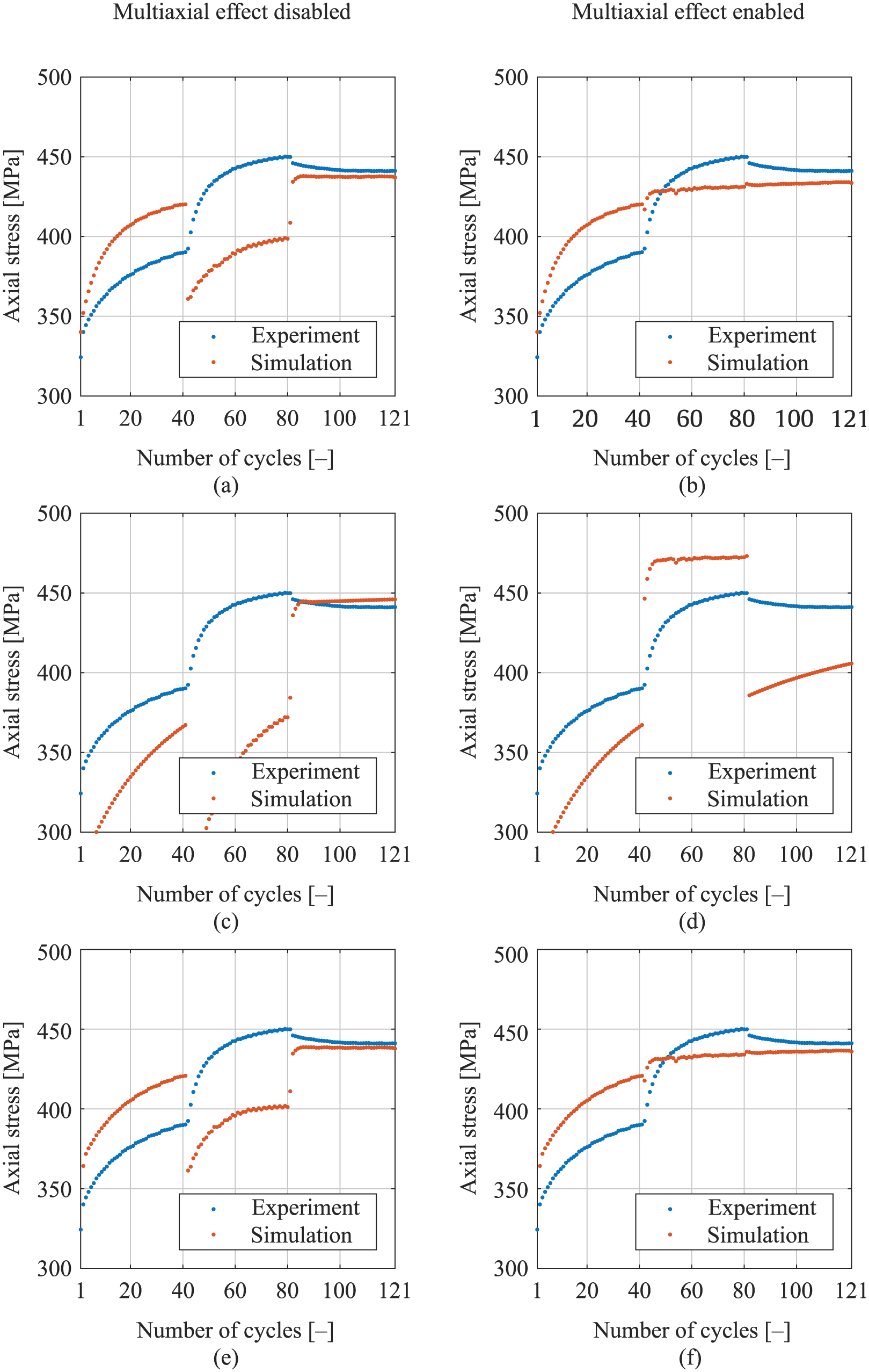
Results for no non-proportional effects are depicted in Figure 11(a), (c) and (e), where the prediction of response is poor. It was better with accounting for the non-proportionality (Figure 11(b), (d), (f)). It should be noted that this improvement was basically achieved by the parameter $δ_{1}$ . The second parameter, $δ_{2}$ , was set to the default value, because it was not influential according to the sensitivity analysis.

Figure 11.

Axial stress against number of cycles for the multiaxial tests when multiaxial parameters were kept the same but only the following set of parameters was used: (a, b) first, (c, d) second and (e, f) third.

A good match was not received for the uniaxial loading (parts I and III of the three-step experiment) because it was not achieved for the solely uniaxial loadings as well (Figure 10) due to the calibration for a wide range of strains. The best match would be achieved for the total strain amplitudes around 1.5%, while the three-step experiment was performed under the total strain amplitude of 0.7%, which is approximately twice smaller.

Conclusion

Code_Aster allows calibrating the advanced cyclic plasticity models simply using the built-in routines. Advanced plasticity models are included in Code_Aster, which enables to account for the strain amplitude magnitude as well as loading non-proportionality. The disadvantage of this open-source code lies in the availability of only two backstresses. This restriction prevents from better capturing of saturated loop shapes, which could be achieved by three or four superimposed backstress terms.^10,41 Nevertheless, it is possible to add more backstresses or create a completely new model since the Code_Aster can be modified. The study demonstrates that with a selected constitutive model, it is crucial to choose a suitable target function according to the intended utilization.

Three sets of parameters were presented. Each set was calibrated under different conditions. The third set of parameters was strongly influenced by the ratcheting parameters; therefore, the simulations with the earlier two sets of parameters were not of acceptable quality regarding the hysteresis loops as well as stress evolution. The third set of parameters provided the best simulations. The trend was excellent although there was a shift for the stress-controlled simulations primarily due to the monotonic response simulation. However, the evolution of peak stress amplitudes under the uniaxial loading was captured well.

In the case of a real component, it would be needed to analyse the operating strain range in service along with the analysis of the multiaxial stress states. More precise calibration can be performed in such a case.

Footnotes

Handling Editor: Daxu Zhang

Declaration of conflicting interests

The author(s) declared no potential conflicts of interest with respect to the research, authorship and/or publication of this article.

Funding

The author(s) disclosed receipt of the following financial support for the research, authorship and/or publication of this article: This work is an output of project NETME CENTRE PLUS (LO1202) created with financial support from the Ministry of Education, Youth and Sports under the ‘National Sustainability Programme I’.

ORCID iD

František Šebek

References

Lin

Liu

Chen

et al . Cyclic plasticity constitutive model for uniaxial ratcheting behavior of AZ31B magnesium alloy. J Mater Eng Perform 2015; 24: 1820–1833.

Fatoba

Akid

Uniaxial cyclic elasto-plastic deformation and fatigue failure of API-5L X65 steel under various loading conditions. Theor Appl Fract Mech 2018; 94: 147–159.

Gróza

Váradi

Total fatigue life analysis of a nodular cast iron plate specimen with a center notch. Adv Mech Eng 2017; 9: 1–11.

Code_Aster Documentation. Clamart: EDF R&D, 2018.

FEMCA Finite Element Method Code Aster, http://www.femca.cz/ (2018, accessed 4 April 2018).

Chaboche

Dang-Van

Cordier

. Modelization of the strain memory effect on the cyclic hardening of 316 stainless steel. In: International Association for Structural Mechanics in Reactor Technology (eds Jaeger

Boley

), Berlin, 13–17 August 1979, p. L11/3 (1–10).

Armstrong

Frederick

. A mathematical representation of the multiaxial Bauschinger effect. Report 4258, 1966, Berkeley Nuclear Laboratories, https://lra.le.ac.uk/bitstream/2381/40272/5/A%20F%202007%20Reproduction.pdf

Voce

The relationship between stress and strain for homogeneous deformations. J Inst Met 1948; 74: 537–562.

Burlet

Cailletaud

Numerical techniques for cyclic plasticity at variable temperature. Eng Comput 1986; 3: 143–153.

10.

Chaboche

JL.

On some modifications of kinematic hardening to improve the description of ratchetting effects. Int J Plast 1991; 7: 661–678.

11.

Bari

Hassan

An advancement in cyclic plasticity modeling for multiaxial ratcheting simulation. Int J Plast 2002; 18: 873–894.

12.

Benallal

Marquis

Constitutive equations for nonproportional cyclic elasto-vicsoplasticity. J Eng Mater Technol 1987; 109: 326–336.

13.

Tanaka

A nonproportionality parameter and a cyclic viscoplastic constitutive model taking into account amplitude dependences and memory effects of isotropic hardening. Eur J Mech A Solids 1994; 13: 155–173.

14.

Hassan

Taleb

Krishna

Influence of non-proportional loading on ratcheting responses and simulations by two recent cyclic plasticity models. Int J Plast 2008; 24: 1863–1889.

15.

Krishna

Hassan

Naceur

et al . Macro versus micro-scale constitutive models in simulating proportional and nonproportional cyclic and ratcheting responses of stainless steel 304. Int J Plast 2009; 25: 1910–1949.

16.

Masing

Eigenspannungen und Verfestigung beim Messing. In: Proceedings of the 2nd international congress of applied mechanics, Zürich, 12–17 September 1926, p.332–335 (in German).

17.

Khutia

Dey

Hassan

An improved nonproportional cyclic plasticity model for multiaxial low-cycle fatigue and ratcheting responses of 304 stainless steel. Mech Mater 2015; 91: 12–25.

18.

Ohno

Wang

JD.

Kinematic hardening rules with critical state of dynamic recovery, Part I: formulation and basic features for ratchetting behavior. Int J Plast 1993; 9: 375–390.

19.

Ohno

Wang

JD.

Kinematic hardening rules with critical state of dynamic recovery, Part II: application to experiments of ratchetting behavior. Int J Plast 1993; 9: 391–403.

20.

Abdel-Karim

Modified kinematic hardening rules for simulations of ratchetting. Int J Plast 2009; 25: 1560–1587.

21.

Abdel-Karim

An extension for the Ohno–Wang kinematic hardening rules to incorporate isotropic hardening. Int J Pres Ves Pip 2010; 87: 170–176.

22.

Meggiolaro

De Castro

JTP

. Non-proportional hardening models for predicting mean and peak stress evolution in multiaxial fatigue using Tanaka’s incremental plasticity concepts. Int J Fatigue 2016; 82: 146–157.

23.

Meggiolaro

De Castro

JTP

A general class of non-linear kinematic models to predict mean stress relaxation and multiaxial ratcheting in fatigue problems – part I: Ilyushin spaces. Int J Fatigue 2016; 82: 158–166.

24.

Meggiolaro

De Castro

JTP

et al . A general class of non-linear kinematic models to predict mean stress relaxation and multiaxial ratcheting in fatigue problems – part II: generalized surface translation rule. Int J Fatigue 2016; 82: 167–178.

25.

Mróz

On the description of anisotropic workhardening. J Mech Phys Solids 1967; 15: 163–175.

26.

Peč

Zapletal

Šebek

et al . Low-cycle fatigue, fractography and life assessment of EN AW 2024-T351 under various loadings. Exp Tech 2019; 43: 41–56.

27.

Chaboche

JL.

A review of some plasticity and viscoplasticity constitutive theories. Int J Plast 2008; 24: 1642–1693.

28.

Hornberger

GM.

An approach to the preliminary analysis of environmental systems. J Environ Manage 1981; 12: 7–18.

29.

Saltelli

Sensitivity analysis for importance assessment. Risk Anal 2002; 22: 579–590.

30.

Rabitz

Systems analysis at the molecular scale. Science 1989; 246: 221–226.

31.

Iooss

Lemaître

A review on global sensitivity analysis methods. In: Dellino

Meloni

(eds) Uncertainty management in simulation-optimization of complex systems. Operations research/computer science interfaces series 59. Boston, MA: Springer, 2015, pp.101–122.

32.

SALib, http://salib.github.io/SALib/ (2018, accessed 1 March 2018).

33.

Sobol’

IM.

Global sensitivity indices for nonlinear mathematical models and their Monte Carlo estimates. Math Comput Simul 2001; 55: 271–280.

34.

Morris

MD.

Factorial sampling plans for preliminary computational experiments. Technometrics 1991; 33: 161–174.

35.

Eiben

Smith

JE.

Introduction to evolutionary computing. In: Rozenberg

Bäck

Eiben

et al . (eds) Natural computing series. Berlin: Springer, 2015.

36.

Islam

Hassan

. Improving simulations for low cycle fatigue and ratcheting responses of elbows. In: Proceedings of the ASME 2016 pressure vessels and piping conference, Vancouver, BC, Canada, 17–21 July 2016, pp. V005T09A012.

37.

Barrett

Ahmed

Menon

et al . Isothermal low-cycle fatigue and fatigue-creep of Haynes 230. Int J Solids Struct 2016; 88–89: 146–164.

38.

Nie

Fan

et al . Cyclic hardening and softening behavior of the low yield point steel BLY160: experimental response and constitutive modeling. Int J Plast 2016; 78: 44–63.

39.

Halama

Markopoulos

Jančo

et al . Implementation of MAKOC cyclic plasticity model with memory. Adv Eng Softw 2017; 113: 34–46.

40.

Zhu

Foletti

Beretta

Probabilistic framework for multiaxial LCF assessment under material variability. Int J Fatigue 2017; 103: 371–385.

41.

Chaboche

JL.

Time-independent constitutive theories for cyclic plasticity. Int J Plast 1986; 2: 149–188.

Automated calibration of advanced cyclic plasticity model parameters with sensitivity analysis for aluminium alloy 2024-T351

Abstract

Keywords

Introduction

Experiments

Modelling methods

Finite element analysis

Sensitivity analysis

Determination of parameters

Results and discussions

Sensitivity analysis results

Strain-controlled tests

Stress-controlled tests

Multiaxial tests

Finite element analysis results

Uniaxial loading

Multiaxial loading

Conclusion

Footnotes

Declaration of conflicting interests

Funding

ORCID iD

References