Sage Journals: Discover world-class research

Abstract

In this article, a dynamic maximal hub location covering problem for a freight transportation system is studied, in which the model has the possibility of having expansion scenarios for future according to the forecasts of increasing demands. Two expansion scenarios are to add up the number of hubs in the network and to add up more carriers. As the markets are involved in the pricing procedure, the model is a bi-level problem which needs more effort to deal with, for which in this work two reformulations based on Karush–Kuhn–Tucker conditions and duality theory are utilized to reformulate the bi-level problem to a single-level one. To solve the model efficiently, a decomposition method is applied and numerical examples are solved to verify the accuracy of the proposed model.

Keywords

Maximal hub covering problem bi-level programming reformulation decomposition

Introduction

Significant progress has been made in the hub location decisions due to recent globalization of freight transportation. Buying goods from other countries is a usual transaction in recent globalization. Transportation companies are enlarging their business in quantity and size to deliver domestic and international orders to customers. To deal with increasing demands and gain more market share, these companies should exploit some strategies in building hub locations for the future. The hub-and-spoke system has become the norm for most major transportation systems because of the numerous advantages such as needless links, needless carriers. Also, the system can sum up the flow in hubs reducing the half loaded carriers, in summary increase productivity and profit. These are from companies’ perspective, but it is also better for customers and markets to use such a system more conveniently. They can get faster services and catch their destination by changing hubs instead of waiting for a long time to reach the direct service. In addition, it would be cheaper than direct service. In this article, this necessity has got attention to develop more practical hub location decision models and give insights to companies cooperating dynamic location decisions in this field. Transportation companies can choose two main expansion strategies to be able to survive in the future competitive business environment. One of the expansion strategies would be to add up the number of hubs, which companies use to carry the demands through. By adding more hubs to the network, companies can connect more nodes and give better services to their customers. Other expansion plan is to buy or lease more carriers to be able to carry more orders. These two expansion plans are included in the mathematical model for the time periods of the planning horizon.

No one can deny the importance of customers in delivery services. If customers are not pleased with the services, they will get service from the rivals and you will lose the profit, reputation, and the market share. As customers’ participation in today’s competitive environment is inevitable, they should participate in the pricing process. This participation of customers is included in the model’s constraints by minimizing the cost paid by customers, which creates a bi-level problem.

In the bi-level optimization, there are two optimization levels: the upper, which is the leader, and the lower, which is the follower. The feasible region of the upper level optimization problem is determined by its own constraints plus the inner optimization problem. The problem leads to generally a nonconvex program and its resolution is so complicated. Even for the simplest bi-level linear programming (LP) models, whose both upper and lower level problems are LP problems, it is known that the problem is theoretically NP-hard.^1,2 Most of the effort in this article is invested in dealing with this inevitable formulation structure.

The model studied in this article focuses on the increasing demand in the future. Expansion plans according to the demand increase are included in the model, in which by participating the customers in the decision-making process the model has become a bi-level model, maximizing the freight company’s profit in the upper level and minimizing the cost paid by customers in the lower level. A Benders decomposition-based method and two reformulations have been conducted to solve the problem and obtain solutions for numerical examples.

Our main contribution is summarized as follows. We develop a dynamic p + q hub location model for freight transportation planning with rational markets. The problem is formulated as a mixed integer bi-level optimization problem. We conduct two approaches to reformulate it into a single-level problem. An efficient Benders decomposition-based algorithm is developed and these approaches are compared from computational experiments.

The reminder of the paper is organized as follows. A literature review is presented. The bi-level problem with rational markets is developed. The bi-level problem is transformed into a single-level problem with a dual based reformulation and Karush–Kuhn–Tucker (KKT) conditions. An efficient method based on Benders decomposition method is proposed to solve the problem. Computational experiments and sensitivity analyses are presented. Finally, in the last section, the paper is concluding with an overview of the findings discussed.

Literature review

Since its introduction in 1970s,^3,4 bi-level optimization has got tremendous research consideration and it has been broadly used in problems with hierarchical decision-making. These hierarchical decision-making problems arise so often in transportation planning and network capacity expansions,^5–7 government policy making,^8,9 and revenue management.^10,11

One of the studies on bi-level models for pricing and revenue management is done by Côté et al.¹¹ They have proposed a first attempt at tackling the airline revenue optimization problem with bi-level models seeking to find a solution for both capacity allocation and pricing sub-problems in a real case study performed at North American airlines. Their formulation integrates a multi-criteria linear assignment model at the second level, whereby customers are segmented into discrete groups, which possess the same valuation for decision criteria. Following this work, Brotcorne et al.¹² presented a bi-level model and a solving method for a problem in the transportation network by setting profit maximizing tariﬀs.

Other previous study is by Garcia-Herreros et al.¹³ who formulated the capacity expansion planning as a bi-level optimization to model decision-making structure, which exists between producers and consumers in the industry. They have formulated their problem as a mixed integer bi-level linear program in which the upper level maximizes the profit of a producer and the lower level minimizes the cost paid by markets. The lower level problem is a linear problem assigning demands of the customers to the cheapest offer of the companies while in the upper level problem, the problem gives solution to expansion planning variables that are mixed integer variables. They also reformulated their bi-level optimization problem as a single-level problem to be able to solve the problem to obtain solutions for their test problems.

Bi-level programming problems are also studied in various applications. Saranwong and Likasiri¹⁴ studied a distribution center problem in the supply chain developing a bi-level model. In the upper level problem, the transportation cost of shipping products from plants to distribution centers is minimized and in the lower level problem, the shipping cost from distribution centers to customers is minimized. They have developed four algorithms to solve computational experiments to investigate the algorithms’ performances.

Gutjahr and Dzubur¹⁵ also proposed a bi-objective, bi-level optimization model for the location of relief DCs in humanitarian logistics. In their problem, an organization that is responsible for preparing health care services seeks to find the location of DCs. In the lower level problem, the customers allocate themselves to the centers with regard to distance and expected supply. They also developed an exact algorithm for determining the Pareto frontier of the problem by combining three solving methods to solve the test problems.

Hemmati and Smith¹⁶ considered the competitive set covering problem as a two-player Stackelberg game that both of the players try to maximize their profit. In this problem, both levels of the problem have binary variables. This kind of problem occurs in situations like facility location games. To solve their problem, they developed a cutting-plane algorithm and showed that their solving procedure has superiority to other available procedures.

A variant of the p-median problem is considered and presented in Ramírez and Vallejo.¹⁷ This variant is based on the assumption that customers are free to choose the located facility that will serve them. The latter decision is made by considering the customers’ preferences toward the facilities. To study this problem, a mathematical bi-level programming formulation is proposed by Ramírez and Vallejo and given the difficulty in solving such bi-level programs, two reformulations have been used for solving the problem. The first reformulation adds constraints and variables to the mathematical model, while the second one adds only constraints. Both reformulations avoid the need to solve an optimization problem parameterized by the upper level variables to find the value of the lower level variables.

Most recently Eltoukhy et al.¹⁸ have studied a joint optimization using a leader–follower Stackelberg game for stochastic operational aircraft maintenance routing problem (as leader) and maintenance staffing problem (as follower). They solved this problem using a bi-level nested ant colony optimization algorithm. Acuña et al.¹⁹ studied a cooperation model between a generating company and several marketers. They studied two schemes in their work: The first scheme is a vertical cooperation between a generation company and several marketers, for which the bi-level optimization was used. The second scheme is a horizontal cooperation between the marketers for which they used Shapley value for profit sharing among markets.

As another recent work in bi-level literature, we can mention the study done by Hajiaghaei and Fathollahifard.²⁰ They have developed a two-stage stochastic bi-level programming model for the distribution network problem in addition to a set of efficient heuristics based on the characteristics of problem. They also did extensive comparisons to examine the performance of their procedures in large networks.

Most recently, Zhang et al.²¹ have examined hub location and plane assignment problems for the air-cargo delivery service. They presented two mixed integer programming models. The difference between these two models is related to how they manage the number of visiting hubs for giving service to each origin–destination pair. Since the problem was NP-hard, they developed a two-stage hybrid algorithm to solve large-scale test problems. In this algorithm, the first stage finds the solution for main variables by heuristics and in the second stage the algorithm finds the solution to the remained variables by a commercial solver. They used real-life data to solve numerical examples to test the efficiency of the models and solving approach.

The above-mentioned works are very noteworthy attempts, especially because of their application to deal with an important real-life fact transportation. To the authors’ best knowledge, there are rare studies on multi-period hub location problem by Gelareh et al.,²² which is one of the first models developed for the uncapacitated multi-period multiple allocation hub location problem, which was first proposed in Gelareh.²³ They have tried to include many features of real life situations in their work, especially features related to land transportation facts. In a precious attempt, they presented a metaheuristic algorithm, which can give high-quality solutions in a reasonable time. They also developed an extension of Benders decomposition technique to solve the test problems and compare the results for both procedures.

Problem definition

The dynamic p + q maximal hub location problem for freight transportation planning with rational markets is described as follows.

Suppose there is a freight company who determines the hub location planning and the required number of transportation vehicles, even operating in air freight transportation or road or other kind of carriers. The carriers that are used by the company to transfer the demand between nodes are called transportation vehicles or carriers in this article. This company uses the hub and spoke system to traverse the flow among nodes and has predefined decisions on the number of established hubs when demand of transportation is given.

The company has some rivals that are operating in the same business environment and even may use the same hubs that our company is using. All rivals are in the same level from our company’s point of view. This means that in total, the whole market share is in two parts: our company’s market share and the rest that goes to the rivals as one amount.

In addition, the company has information about the increasing demand in the future and is eager to gain benefit through establishing some expansion plans. This expectation on the future increasing demand and the necessity to gain advantage of this situation has led to study the problem as a dynamic model.

The company has some dominant customers that have great power and can control the prices by sourcing the demand to the rivals. This ability of the customers is included in the constraints of the model that has made the model to be a bi-level one. The freight company sells the service of flow by sales price depending on origin and destination and customers will buy the service with the sales price. The freight company makes its decisions in the upper level problem as the leader and the follower in the lower level represents the response of markets that select freight companies as providers, with the unique interest of satisfying their demands at the lowest cost. The leader in the first step defines its price and in the next step, the follower reacts according to the prices of the available companies to choose the cheapest one.

The nodes of the network are shown by $N = R \cup U = {1, \dots, n}$ , U refers to the set of nodes that are controlled by the company while R refers to the set of nodes controlled by the rivals. $i, j, k, m$ are used to refer to the nodes of this graph in which $i, j$ refer to spokes and $k, m$ refer to hubs. The markets place an order to be traversed from origin node i to destination node $j .$ The company has freedom in choosing the hubs to carry this order and also the order can be divided and carried using different hubs and seeks to maximize the flow carried by carriers to maximize the income. If the company does not have enough capacity or possibility to transport the order and the order has been already booked, then the company can outsource it to a sister company. It has been achieved using the parameter $o_{km}$ that indicates 1 if there are outsourcing services between nodes i and j and 0 otherwise.

Up to here our problem is a $p + q$ dynamic multi-allocation maximal hub location problem (p is the number of hubs to be utilized at the beginning of the planning horizon and the q is the number of hubs that the company is going to add to its current hubs as expansion plan) in which markets are rational and have the possibility to select their providers according to their own interest, that is, price.

Given the information of travel time (distance) between n nodes, the price paid by customers, demand of transportation and capacity of the carriers, fixed costs of locating a hub, market share for the competitors, rivals’ hub location, the number of carrier type l in the link $k - m$ for rivals, binary parameter $g_{ikmj} \in {0, 1}$ whether or not the demand of origin–destination $i - j$ can be served according to the time (distance) needed to traverse from hubs k and m depending on the discount factor $α$ , the number of hubs at the beginning of planning horizon, the number of hubs as expansion hubs, deadline traveling time (or distance), that is used as covering criteria in which if the time (distance) needed to travel from an origin to its destination through assigned hubs is more than this deadline, the related demand will remain unserved, the decisions to be made in this model are: In the upper level problem; which hubs are going to be opened at the start of planning horizon, and which hubs will be located in the future periods? Which hubs are operating in each period? Other decisions are related to the number and type of carriers in each period. In addition, in the lower level problem, the amount of flow that is going to be carried through the hubs would be determined.

Note 1. The company’s expansion plan is about opening new hubs or buying/leasing new carriers in future periods. Furthermore, when the company opens a hub either at the start of planning horizon or in expansion allowed periods, it cannot close them through the planning horizon.

Note 2. The company and the rivals may share hubs or not. For example, two or more companies may benefit hub k but it can be either the rival company or our company who is using the hub m.

Important note 3. The markets are involved in the pricing decision of the carried flow by having the power to choose the cheapest company. This rational behavior of the markets, that is, minimizing their costs by selecting the cheapest service, is included in the constraints of the problem, which creates a bi-level optimization problem. In this model, the leader (the freight company) maximizes its profit, while the follower (the market) in the lower level problem minimizes the price paid by them, with regard to demand, capacity of hubs and carriers and market share constraints.

Illustrative example

Figure 1(a) and (b) depicts two feasible solutions of an instance where the number of nodes $N = 10$ , the number of transportation vehicle types $l = 4$ , the number of initial hubs $p = 2$ , the number of expansion hub $q = 2$ . This example is studied in the total planning horizon $T = 4$ , but here just the solutions for $t = 1$ and $t = 3$ are depicted. The circles are market nodes and the green hexagonal are used to refer to the companies established hubs; the yellow one is for rival’s hubs and the dark green is for the hubs that are used by both our company and rival. One can track the flow by the colors of the edges; different colors are used for each demand of customers to be carried from an origin node to its destination node. Also the shapes trapezoid, rectangle, square, and triangle refer to different kinds of carriers. These carriers differ in capacity and other efficiency factors. In Figure 1(a), the rival’s hub is located on node 5 and the demand of node 4 is just covered by this rival. Hub 10 is utilizing by both companies, and hub 6 is managed by our company. For nodes that carry large flow, more than one vehicle is assigned. In Figure 1(b), because of predicted increasing demand, the company decides to have an expansion plan and increase the number of hubs to four and also buy/lease more carriers. In this model, because the company does not have any information about the rival’s plan, no change has happened in his hubs. In this period, the company has also entered in the market number 4 and the flow of this market is carried by hub 3. The hubs are interconnected and a huge amount of flow is traversing through them. It should be noted that in this illustration, the distance between nodes is not considered and this is just a schematic try to have a view of the model application.

Figure 1.

Two feasible solutions of an instance where $N = 10, l = 4, p = 2, q = 2$ : (a) t = 1 and (b) t = 3.

Mathematical formulation

The definition of the model parameters and decision variables are listed in the following.

Indices

$i, k, m, j$ Index of nodes.

l Index of transportation vehicle type. Index $l_{0}$ is exclusively used to represent the outsourcing carrier no matter what specific type it is.

t Index of planning horizon, t = 0 refers to the start of planning horizon that initial hubs are allowed. $t = 1, \dots, T$ is used to refer to periods that expansion is allowed in them.

Parameters

$c_{ij}$ Travel time (distance) of each pair of n nodes connected by an arc $(i, j)$ .

$re v_{ijt}$ Price paid by the market for carrying 1 kg weight from node i to node j in period t.

$d_{ijt}$ Markets demand to be carried from origin i to destination j at period t.

$ca p_{l}$ The capacity of transportation vehicle type l.

$cap c_{k}$ The capacity of node k as chosen to be hub.

$E_{k}$ Fixed cost of locating a hub at node k at the beginning of the planning horizon.

$F_{kt}$ Fixed cost of locating a hub at node k at period t.

$A_{kmlt}$ Hourly transportation cost of using transportation vehicle type l, from node k to node m at period $t .$

$F'_{kt}$ Operational cost of hub located at node k at period t.

$MS h_{r}$ Market share for the rival company r.

$x r_{kml}$ The number of carrier type l in the link $k - m$ for rival.

$α$ Discount factor to pass by hubs on the route of $i - j$ , where $0 \leq α \leq 1$ .

p The number of hubs at the start of planning horizon.

q The number of hubs decided as expansion.

$β$ The deadline traveling time (distance) from node i to node j, set to assess the coverage.

$o_{km}$ 1 if there are outsourcing services between nodes i and j, 0 otherwise.

$bud g_{t}$ Available budget at period t.

$g_{ikmj}$ Binary parameter, which indicates whether the origin–destination pair ( $i - j$ ) distance using hubs $k - m$ can be covered by $β$ as

$g_{ikmj} = {\begin{matrix} 1 if c_{ik} + α c_{km} + c_{jm} \leq β \\ 0 otherwise \end{matrix}$

Decision variables

Upper level decision variables

$H_{k}$ Binary variable, 1 if node k is selected as an initial hub at the start of planning horizon.

$v_{kt}$ Binary variable, 1 if node k is selected as an expansion hub at period t.

$h_{kt}$ Binary variable, 1 if node k is operating as a hub at period t.

$x_{kmlt}$ The number of carrier type l in the link $k - m$ at period t. $x_{km l_{0} t}$ can be interpreted as outsourcing amount on link $k - m$ .

Lower level decision variables

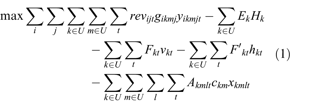
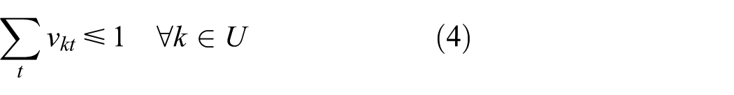
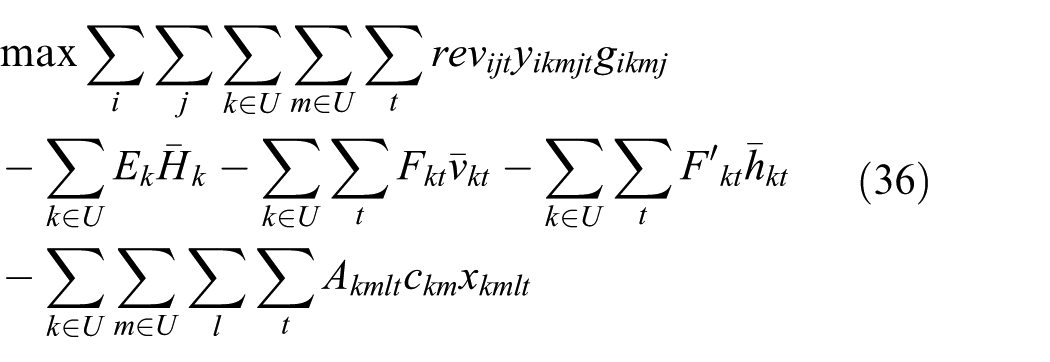
$y_{ikmjt}$ The amount of flow carried from node i to node j through hubs $k - m$ at period $t .$

The problem is formulated as a bi-level optimization problem in equations (1)–(22). In the upper level problem, the freight company is going to choose the location of hubs and the number of carriers with the objective of maximizing the profit. In the lower level problem, given the cost of different companies for carrying the demand, the customers choose the cheapest company to carry their requests. It should be highlighted that the upper objective takes into account the prices of the main studying company while the lower objective contains the prices offered from all companies performing in the business. The first term in the objective function in equation (1) maximizes the income gained from carrying flow through the hubs that are controlled by the leader, while the second and third terms are for the fixed cost of establishing initial hubs and expansion hubs, the fourth term is related to operational cost of hubs, and the fifth term is for the transportation cost of the self-owned carriers and outsourcing. Constraint (2) restricts the primary number of established initial hubs to be p. Constraint (3) ensures that the number of expansion hubs to be q. Constraints (4) imply that each expansion hub can be opened only once throughout the planning horizon. Constraints (5) and (6) together enforce that once a hub is selected as an initial or expansion hub, it should be used for whole time periods. Constraints (7) state that no carrier can be assigned to link $k - m$ unless one of these nodes is operating as hub (M is a large positive number). Constraints (8) mean that unless there is not outsourcing service for the link $k - m$ , no outsourcing is allowed for that link. Constraints (9) are related to this assumption that usually the number of the carriers operating in backward direction is the same as that in the forward direction. Constraints (10) are for the budget limitation of buying or leasing the carriers. Constraints (11) and (12) define the variables in the upper level problem as binary and positive integer variables.

The objective function (13) in the lower level problem minimizes the cost paid by the markets. Constraints (14) and (15) imply that no flow can be carried through nodes unless they use hub/hubs. M used in these constraints is a large positive number. Constraints (16) imply that the total flow from node i to node j at each period t should be equal to the demand of that origin and destination. Constraints (17) make sure that the total capacity of employed carriers should not be violated. In this constraint, the left-hand side is the total flow occurring on link $k - m$ utilizing by our company, including the amount $\sum_{i} \sum_{j} y_{ikmjt}$ that transfers from other $i - j$ pairs, and the amount $\sum_{o \in N} \sum_{d \in N} (y_{kmodt} + y_{odkmt})$ that is transferred to or from other node pairs, these pairs are shown by o and d. The right-hand side is the total capacity of the carriers employed to link $k - m$ utilizing by our company. Constraints (18) state that the total flow for the rivals’ hubs could at most be equal to the situation it had since past. In addition, constraints (19) state that the amount of flow carried through the rivals’ hub should be equal or less than their market share of the demand. Constraints (20) and (21) make sure that the total capacity of established hubs should not be violated. It worth noting that all variables in upper level problem take discrete values while the variables in lower level problem have continuous variables. Constraints (22) enforce the decision variables to be non-negative. The nature of the model variables plays an important role in reformulation techniques of bi-level problems. In the bi-level reformulation literature, there are many papers studying models having different kinds of variables in upper level and lower level problem theoretically and practically.

\begin{matrix} max \sum_{i} \sum_{j} \sum_{k \in U} \sum_{m \in U} \sum_{t} re v_{ijt} g_{ikmj} y_{ikmjt} - \sum_{k \in U} E_{k} H_{k} \\ - \sum_{k \in U} \sum_{t} F_{kt} v_{kt} - \sum_{k \in U} \sum_{t} {F'}_{kt} h_{kt} \\ - \sum_{k \in U} \sum_{m \in U} \sum_{l} \sum_{t} A_{kmlt} c_{km} x_{kmlt} \end{matrix}

(1)

\sum_{k \in U} H_{k} = p

(2)

\sum_{k \in U} \sum_{t} v_{kt} = q

(3)

\sum_{t} v_{kt} \leq 1 \forall k \in U

(4)

h_{kt} \geq H_{k} + v_{kt} \forall k \in U, t

(5)

h_{kt} \geq h_{kt - 1} \forall k \in U, t

(6)

x_{kmlt} \leq M (h_{kt} + h_{mt}) \forall k \in U, m \in U, t

(7)

x_{km l_{0} t} = 0 \forall k \in U, m \in U, l_{0}, where o_{km} = 0

(8)

x_{kmlt} = x_{mklt} \forall k \in U, m \in U, l \neq l_{0}, t

(9)

\sum_{k \in U} \sum_{m \in U} \sum_{l} \cos t_{l} x_{kmlt} \leq bud g_{t} \forall t

(10)

H_{k}, v_{kt}, h_{kt} \in {0, 1}

(11)

x_{kmlt} \in Z^{+}

(12)

min \sum_{i} \sum_{k \in U \cup R} \sum_{m \in U \cup R} \sum_{j} \sum_{t} re v_{ijt} y_{ikmjt} g_{ikmj}

(13)

y_{ikmjt} \leq M h_{kt} \forall i, j, k \in U, m \in U, t

(14)

y_{ikmjt} \leq M h_{mt} \forall i, j, k \in U, m \in U, t

(15)

\sum_{k \in U \cup R} \sum_{m \in U \cup R} y_{ikmjt} = d_{ijt} \forall i, j \in U \cup R, t

(16)

\begin{matrix} \sum_{i} \sum_{j} y_{ikmjt} + \sum_{o \in N} \sum_{d \in N} (y_{kmodt} + y_{odkmt}) \\ \leq \sum_{l} ca p_{l} x_{kmlt} \forall k \in U, m \in U, t \end{matrix}

(17)

\begin{matrix} \sum_{i} \sum_{j} y_{ikmjt} + \sum_{o \in N} \sum_{d \in N} (y_{kmodt} + y_{odkmt}) \\ \leq MS h_{r} \sum_{l} ca p_{l} x r_{kml} \forall k \in R, m \in R, t \end{matrix}

(18)

\sum_{k \in R} \sum_{m \in R} y_{ikmjt} \leq MS h_{r} d_{ijt} \forall i, j \in U \cup R, t

(19)

\sum_{i} \sum_{m \in U} \sum_{j} y_{ikmjt} \leq cap c_{k} h_{kt} \forall k \in U, t

(20)

\sum_{i} \sum_{k \in U} \sum_{j} y_{ikmjt} \leq cap c_{m} h_{mt} \forall m \in U, t

(21)

y_{ikmjt} \in R^{+} \forall i, j, k and m \in U \cup R, t

(22)

Reformulation as a single-level optimization problem

In particular, bi-level programs have significant importance due to the fact that they have been widely used in the Stackelberg games which involve two interacting players in different levels with different objectives using a set of common resources. The goal of a bi-level optimization technique is then to find the lower level optimal solutions and then search for the optimal solution for the upper level optimization tasks. The broader adoption of bi-level frameworks has only been limited by computational challenges while optimization problems with a bi-level nature are hard to solve. A bi-level program with a convex and regular lower level can be transformed into a single-level optimization problem using its optimality conditions. We derive two single-level reformulation for the modified problem to be able to solve them and compare the results of each reformulation. First one is reformulation based on duality theory and the second one is obtained by KKT conditions.

Dual based reformulation

To conduct this reformulation, the upper level problem remains unchanged and the reformulation is performed on lower level problem. For this reformulation, the equivalent dual problem of the lower level problem has to be obtained. The dual constraints will be added to the constraints of the lower problem and the objective functions of primal and dual problem should be equated. $v 1_{ikmjt}, v 2_{ikmjt}, v 3_{ijt}, v 4_{kmt}, v 5_{kmt},$ $v 6_{ijt}, v 7_{kt},$ and $v 8_{mt}$ are the dual variables of the lower level constraints presented in equations (14)–(21), respectively. In this reformulation, the constraints of the upper level problem (equations (1)–(12)) remain unchanged.

Equations (1)–(12) and (14)–(22)

\begin{matrix} \sum_{i} \sum_{k \in U \cup R} \sum_{m \in U \cup R} \sum_{j} \sum_{t} re v_{ijt} y_{ikmjt} g_{ikmj} \\ = \sum_{i} \sum_{j} \sum_{t} d_{ijt} v 3_{ijt} \\ - \sum_{i} \sum_{j} \sum_{t} MS h_{r} d_{ijt} v 6_{ijt} \\ - \sum_{i} \sum_{k \in U} \sum_{m \in U} \sum_{j} \sum_{t} M v 1_{ikmjt} h_{kt} \\ - \sum_{i} \sum_{k \in U} \sum_{m \in U} \sum_{j} \sum_{t} M v 2_{ikmjt} h_{mt} \\ - \sum_{k \in U} \sum_{m \in U} \sum_{l} \sum_{t} ca p_{l} v 4_{kmt} x_{kmlt} \\ - \sum_{k \in R} \sum_{m \in R} \sum_{l} \sum_{t} ca p_{l} v 5_{kmt} x r_{kml} \\ - \sum_{k \in U} \sum_{t} v 7_{kt} h_{kt} cap c_{k} \\ - \sum_{m \in U} \sum_{t} v 8_{mt} h_{mt} cap c_{m} \\ v 1_{ikmjt} + v 2_{ikmjt} - v 3_{ijt} + v 4_{kmt} + v 5_{kmt} + v 6_{ijt} + v 7_{kt} + v 8_{mt} \\ \geq - re v_{ijt} g_{ikmj} \end{matrix}

(23)

\forall i, k \in U \cup R, m \in U \cup R, j, t

(24)

v 1_{ikmjt}, v 2_{ikmjt}, v 4_{kmt}, v 5_{kmt}, v 6_{ijt}, v 7_{kt}, v 8_{mt} \in R^{+} v 3_{ijt} \in R

(25)

By equating the primal and dual objective functions of the lower level problem in equation (23), the strong duality is enforced. The feasibility of primal and dual problems should be guaranteed in the reformulation. This important fact for primal is ensured by keeping constraints (14)–(22) and for the dual problem is ensured by adding constraints (24).

By the reformulation, it is obvious that equation (23) is nonlinear that yields a mixed integer nonlinear program (MINLP). Fortunately, we can linearize it by popular techniques known as linearizing the product of binary and continues variables, in which before that another reformulation should be applied to convert the integer variables to an expression, which is a summation of binary variables. Both conversion techniques are available in operations research related material. By linearizing the nonlinear expressions in equation (23), the bi-level problem is converted into a single-level problem and solution procedures can be applied to solve the problem.

Reformulation using KKT conditions

An appealing way to deal with general bi-level problems is the so-called KKT approach, where the lower level constraints, that its variables are a global minimizer of the lower level program, are first relaxed to the conditions that the optimal variables of the lower level problem are a local minimizer for that lower level problem. The main purpose of the KKT approach is to find (local) minimizers of the original bi-level program by computing (local) minimizers of the relaxation obtained from KKT equivalent.^24,25 This is the original reformulation for bi-level problems that the lower level is an LP to replace the lower level problem with its KKT conditions. The resulting reformulation is presented in the following

Equations (1)–(12), (14)–(22), and (25)

\begin{matrix} re v_{ijt} g_{ikmj} + v 1_{ikmjt} + v 2_{ikmjt} + v 3_{ijt} + v 4_{kmt} + v 5_{kmt} \\ + v 6_{ijt} + v 7_{kt} + v 8_{mt} - v 9_{ikmjt} = 0 \end{matrix}

\forall i, k \in U \cup R, m \in U \cup R, j, t

(26)

v 1_{ikmjt} (y_{ikmjt} - M h_{kt}) = 0 \forall i, k \in U, m \in U, j, t

(27)

v 2_{ikmjt} (y_{ikmjt} - M h_{mt}) = 0 \forall i, k \in U, m \in U, j, t

(28)

\begin{matrix} v 4_{kmt} (\sum_{i} \sum_{j} y_{ikmjt} + \sum_{o \in N} \sum_{d \in N} (y_{kmodt} + y_{odkmt}) - \sum_{l} ca p_{l} x_{kmlt}) \\ = 0 \forall k \in U, m \in U, t \end{matrix}

(29)

\begin{matrix} v 5_{kmt} (\sum_{i} \sum_{j} y_{ikmjt} + \sum_{o \in N} \sum_{d \in N} (y_{kmodt} + y_{odkmt}) - MS h_{r} \sum_{l} ca p_{l} x r_{kml}) \\ = 0 \forall k \in R, m \in R, t \end{matrix}

(30)

v 6_{ijt} (\sum_{k \in R} \sum_{m \in R} y_{ikmjt} - MS h_{r} d_{ijt}) = 0 \forall i, j \in U \cup R, t

(31)

v 7_{kt} (\sum_{i} \sum_{m \in U} \sum_{j} y_{ikmjt} - cap c_{k} h_{kt}) = 0 \forall k \in U, t

(32)

v 8_{mt} (\sum_{i} \sum_{k \in U} \sum_{j} y_{ikmjt} - cap c_{m} h_{mt}) = 0 \forall m \in U, t

(33)

v 9_{ikmjt} y_{ikmjt} = 0 \forall i, j, k and m \in U \cup R, t

(34)

v 9_{ikmjt} \in R^{+}

(35)

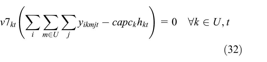
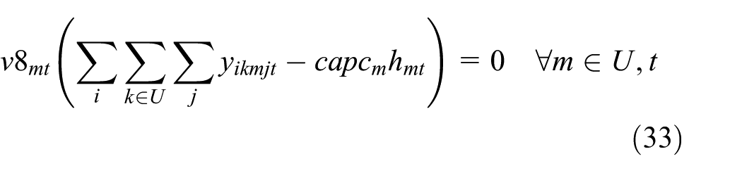
The upper level problem is kept unchanged as shown in equations (1)–(12). In KKT approach, there are two main conditions as stationary conditions and complementary conditions. Constraints (26) are the stationary conditions for the lower level, where constraints (27)–(34) represent the complementary conditions corresponding to inequalities (14), (15), and (17)–(22). Note that in KKT conditions, the constraints representing the domain of the continuous variables are treated as constraints and complementary conditions must be written for these constraints either.

By this reformulation, the bi-level model is converted to a single-level model. But the disadvantage that appears in this reformulation is the nonlinear complementary constraints. To avoid the nonlinear complementary constraints, we rewrite equations (14), (15), and (17)–(21) as equality constraints using the slack variables and then use the big-M method to express either constraints (14), (15), and (17)–(21) are active or the corresponding multipliers are zero. Similarly, the same big-M reformulation should be done for constraint (34).

This process has to be fulfilled for all complementary conditions and the necessary constraints for all of them should be included in the model. By this procedure, we can get rid of nonlinear complementary conditions. The result of this replacement for complementary constraints is a single-level mixed integer linear problem that can be solved by solvers.

Efficient solution procedure

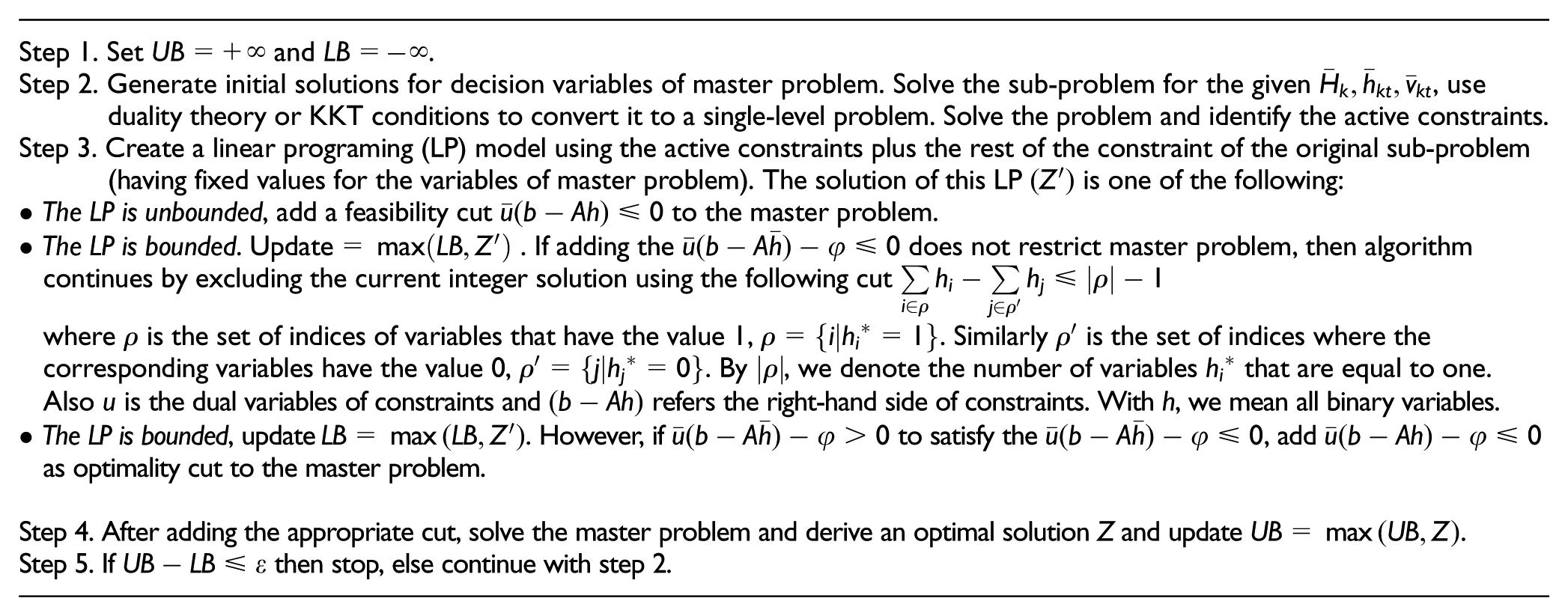
To solve the single-level problem, which is obtained in the previous section, the general-purpose mixed integer programming solvers can solve small problems up to 10 nodes. This fact shows the necessity to propose or apply other available solving methods. As the decision variables can easily be classified into two categories: integer and continues variables; a solving method based on Benders decomposition is possible to be applied to solve the problem.

There are some decomposition techniques in literature that were proposed based on the Benders decomposition method. One of these methods is proposed by Saharidis and Ierapetritou²⁶ for mixed integer bi-level linear problems. In this method, after dividing the problem into sub-problem and master problem, Saharidis and Ierapetritou convert the bi-level sub-problem into single level using KKT conditions. Then similar to Benders decomposition method, the master problem and sub-problem are solved and they are synced in each iteration.^27,28

For the conversion process of the bilevel subproblems into a single-level one, both duality-based method and KKT method are used. The algorithm is as follows:

Step 1. Set

UB = + \infty

and

LB = - \infty

.
Step 2. Generate initial solutions for decision variables of master problem. Solve the sub-problem for the given

{\bar{H}}_{k}, {\bar{h}}_{kt}, {\bar{v}}_{kt}

, use duality theory or KKT conditions to convert it to a single-level problem. Solve the problem and identify the active constraints.
Step 3. Create a linear programing (LP) model using the active constraints plus the rest of the constraint of the original sub-problem (having fixed values for the variables of master problem). The solution of this LP

(Z')

is one of the following:
• The LP is unbounded, add a feasibility cut

\bar{u} (b - Ah) \leq 0

to the master problem.
• The LP is bounded.

Update = max (LB, Z')

. If adding the

\bar{u} (b - A \bar{h}) - φ \leq 0

does not restrict master problem, then algorithm continues by excluding the current integer solution using the following cut

\sum_{i \in ρ} h_{i} - \sum_{j \in ρ'} h_{j} \leq | ρ | - 1

where

ρ

is the set of indices of variables that have the value 1,

ρ = {i | {h_{i}}^{*} = 1}

. Similarly

ρ'

is the set of indices where the corresponding variables have the value 0,

ρ' = {j | {h_{j}}^{*} = 0}

. By

| ρ |

, we denote the number of variables

{h_{i}}^{*}

that are equal to one. Also u is the dual variables of constraints and

(b - Ah)

refers the right-hand side of constraints. With h, we mean all binary variables.
• The LP is bounded,

update LB = max (LB, Z')

. However, if

\bar{u} (b - A \bar{h}) - φ > 0

to satisfy the

\bar{u} (b - A \bar{h}) - φ \leq 0

, add

\bar{u} (b - Ah) - φ \leq 0

as optimality cut to the master problem.
Step 4. After adding the appropriate cut, solve the master problem and derive an optimal solution Z and update

UB = max (UB, Z)

.
Step 5. If

UB - LB \leq ε

then stop, else continue with step 2.

Sub-problem

The sub-problem is derived by fixing decision variables $H_{k}, h_{kt}, v_{kt}$ with ${\bar{H}}_{k}, {\bar{h}}_{kt}, {\bar{v}}_{kt}$ in inner problem and adding the terms of the upper level objective function which contains the expressions related to the variables $y_{ikmjt}$ and $x_{kmlt}$ . As the sub-problem would be a bi-level problem, to convert it to a single-level problem, both the dual based and KKT condition reformulation will be used and the obtained results would be compared. Therefore, the sub-problem is

\begin{matrix} max \sum_{i} \sum_{j} \sum_{k \in U} \sum_{m \in U} \sum_{t} re v_{ijt} y_{ikmjt} g_{ikmj} \\ - \sum_{k \in U} E_{k} {\bar{H}}_{k} - \sum_{k \in U} \sum_{t} F_{kt} {\bar{v}}_{kt} - \sum_{k \in U} \sum_{t} {F'}_{kt} {\bar{h}}_{kt} \\ - \sum_{k \in U} \sum_{m \in U} \sum_{l} \sum_{t} A_{kmlt} c_{km} x_{kmlt} \end{matrix}

(36)

s.t: (7)–(10) and (12)–(22).

To be able to solve the sub-problem by decomposition method, the integer variables $x_{kmlt}$ are relaxed to be positive continues ones.

Master problem

The master problem is the upper level problem, which optimizes variables $H_{k}, h_{kt}, v_{kt}$ . Note that in solving process, the necessary cuts should be added to the master problem

\min \sum_{k \in U} E_{k} H_{k} + \sum_{k \in U} \sum_{t} F_{kt} v_{kt} - \sum_{k \in U} \sum_{t} F'_{kt} h_{kt} - φ

(37)

s.t. equations (2)–(6) and (11).

The value $φ$ is the value for terms related to variables ${\bar{y}}_{ikmjt}$ and ${\bar{x}}_{kmlt}$ in the sub-problem.

Computational results

In this section, we show some numerical examples to evaluate the model and solving methods’ efficiency. Most of the main parameters of the problem such as travel time (distance), demand, hub capacities and costs, which are used as an example to solve, are from a real case in Turkey.²⁹ Other parameters such as carrier capacities and hourly transportation cost of carriers are taken from Zhang et al.²¹ Other parameters are included in Table 1. This should be marked that for parameters $A_{kmlt}$ and $re v_{ijt}$ to save space, we just include the minimum and maximum values using [ $mi n_{ij}$ , $ma x_{ij}$ ] format (there are four sets of ([ $mi n_{ij}$ , $ma x_{ij}$ ] values at each period t for $A_{kmlt}$ , which refers to each l). We set the other parameters: $α = 0.7$ , p = 2, q = 2, l = 4, T = 4, and β = 1300 for 10 nodes instance. Furthermore, $MS h_{r} = 0.3$ and for the availability of outsource service parameter $o_{km}$ , we have set the condition that this service is available for demands lower than 30,000. All the problems are coded in GAMS 24.1 CPLEX 24.1.2 solver and run on a personal computer of Core i7, 3.40 GHz, 8 GB RAM.

Table 1.

Parameters for the instance of 10 nodes.

Parameter	Values
$E_{k}$	{4790, 7748, 4738, 6716, 5653, 3104, 3265, 6521, 5497, 3618}
$F_{kt}$	t = 1 {6418, 10383, 6349, 8999, 7575, 4160, 4375, 8738, 7366, 4848} t = 2 {7328, 11855, 7249, 10276, 8649, 4750, 4995, 9976, 8410, 5535} t = 3 {7951, 12862, 7865, 11149, 9384, 5153, 5419, 10824, 9125, 6006} t = 4 {8094, 13095, 8007, 11351, 9553, 5246, 5517, 11020, 9290, 6114}
$F'_{kt}$	t = 1 {1284, 2077, 1270, 1800, 1515, 832, 875, 1747, 1473, 970} t = 2 {1466, 2371, 1450, 2055, 1730, 950, 999, 1995, 1682, 1107} t = 3 {1590, 2572, 1573, 2230, 1877, 1031, 1084, 2165, 1825, 1201} t = 4 {1619, 2619, 1601, 2270, 1911, 1049, 1103, 2204, 1858, 1223}
$A_{kmlt}$	t = 1 {[1.29, 1.47], [1.12, 1.29], [0.6, 0.77], 0.0001} t = 2{[1.32, 1.49], [1.14, 1.32], [0.61, 0.79], 0.0001} t = 3{[1.34, 1.52], [1.16, 1.34], [0.62, 0.80], 0.0001} t = 4{[1.38, 1.56], [1.19, 1.38], [0.64, 0.82], 0.0001}
$ca p_{l}$	{40000, 28000, 14000, $1}$
$bud g_{t}$	{31,717,470, 38,432,670, 35,503,750, 33,011,380}
$re v_{ijt}$	t = 1 [3.9, 23.5] t = 2 [4.02, 23.7] t = 3 [4.1, 24.1] t = 4 [4.2, 24.6]
$x r_{kml}$	$x r_{10, 3, 1} = 1$ , $x r_{3, 5, 2} = 1, x r_{5, 6, 1} = 1$ , others = 0

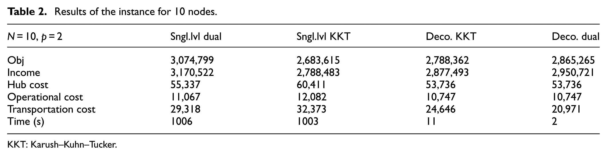
The first problem to solve has 10 nodes in the network, the number of hubs at the start of planning horizon would be two, and we are allowed to have two more hubs after second period. The results for this problem are included in Table 2. In this table, the first and second columns contain the results for single-level reformulations based on duality theory and KKT conditions, respectively, also, third and fourth columns contain the results obtained from the decomposition methods using the duality theory and KKT conditions in reformulating the sub-problem, respectively. The first row illustrates the objective value and the other rows contain the different terms in the objective function, to have a better insight of them. The last row illustrates the computational time to solve each problem in seconds.

Table 2.

Results of the instance for 10 nodes.

N = 10, p = 2	Sngl.lvl dual	Sngl.lvl KKT	Deco. KKT	Deco. dual
Obj	3,074,799	2,683,615	2,788,362	2,865,265
Income	3,170,522	2,788,483	2,877,493	2,950,721
Hub cost	55,337	60,411	53,736	53,736
Operational cost	11,067	12,082	10,747	10,747
Transportation cost	29,318	32,373	24,646	20,971
Time (s)	1006	1003	11	2

KKT: Karush–Kuhn–Tucker.

According to the results in Table 2, we can conclude that the dual based single-level reformulation has a better functionality, as its solution is more than the KKT reformulation and the solution value is closer to the solution obtained from decompositions. Between the two decomposition methods, the decomposition that has used duality theory has produced better solution in much less time. This problem is solved for some changes in parameters of the maximum allowed coverage distance in addition to 25% increase and decrease on hubs and carriers capacities. The results are illustrated in Table 3 and Figure 2.

Table 3.

Results of some sensitivity examinations.

N = 10, p = 2		Sngl.lvl dual	Sngl.lvl KKT	Deco. KKT	Deco. dual
1	Main	3,074,799	2,683,615	2,788,362	2,865,265
2	β = 1500	3,439,385	2,854,862	3,355,062	3,362,556
3	C.cap–25%	2,402,696	1,649,895	2,135,054	2,158,608
4	C.cap +25%	3,584,927	2,838,918	3,123,215	3,388,515
5	H.cap –25%	3,004,058	2,639,804	2,780,162	2,858,275
6	H.cap +25%	3,089,888	2,719,115	2,793,311	2,869,459

KKT: Karush–Kuhn–Tucker.

Figure 2.

Results of some sensitivity examinations.

The results in Table 3 and Figure 2 show the same trends in Table 2. Comparing single-level reformulations (third and fourth column), it is obvious that reformulation based on duality theory has apparent superiority to KKT reformulation method. The same conclusion can be set off from comparing decomposition methods using both KKT and Duality reformulation in which decomposition method using duality reformulation produces better objective values. For all test problems of sensitivity analysis, the dual reformulation approach has the maximum objective value and KKT reformulation has the minimum objective value for all instances.

However, the main purpose of this table is to evaluate the model performance by running some sensitivity analysis. All approaches have the same level of efficiency regarding objective function value, being able to find reasonable values for test problems. When the coverage distance increased and the capacity of hubs and carries are increased, the objective value is supposed to be increased and by reducing the capacities, the objective value is supposed to be reduced and the solutions in Table 3 confirms these assumptions.

According to Table 3 and regarding the increasing the coverage parameter from 1300 to 1500, the objective value of all procedures have been changed such that they are assumed to, due to the fact that by increasing the coverage parameter more nodes may be covered and consequently the profit will be increased. The same results are obvious for cases increasing capacity of carriers and hubs, and on the contrary, reducing the capacity has resulted to less values of the objective function. In addition, comparing the impact of differences in capacities, it can be implied that increasing the carriers’ capacity has more impact on solutions rather than hub capacities. For example, in the reformulation based on dual theory, the difference of values obtained from carrier capacities increasing by 25% and the main objective value (C.cap +25%)—(Main) is about 510,128 while this difference is about 15,089 for hubs capacity (H.cap +25%)—(Main). The same results are also obtained by other approaches which assure that if the company wants to choose between increasing the capacity of carriers or hubs, the priority is with increasing the capacity of carriers.

Single-level reformulations were not able to solve problems more than 10 nodes, so that no more comparison was possible to conduct, especially for comparing reformulation and decomposition both based on duality theory. That is the reason that the rest of the comparisons are performed on decompositions based on KKT and duality theory. In the similar way, some test problems are solved increasing the number of the nodes in the network and results are shown in Table 4. The rows in this table refer to different problems solved. For example, the first row is related to the problem having 15 nodes in which $p = 3$ hubs have to be located in the first period. In all examples, the number of new hubs to be located as expansion plan is fixed to $q = 2$ . Both reformulations were unable to solve the examples, so that just the solutions of two decompositions exist in the table. The decomposition method which uses the KKT condition to reformulate the bi-level sub-problems into a single-level one (first and second column) solved the problem much longer than the duality-based decomposition has (the third and fourth column). Considering the computational efforts, it is apparent that duality-based decomposition has a much better performance than KKT-based decomposition. Also, KKT-based decomposition method could not find the solution to problems more than 20 nodes; however, the dual based decomposition could obtain the solution for problems up to 30 nodes at an acceptable computational time. Comparing the objective value for 15 and 20 nodes of both decompositions, both of them have relatively acceptable values, although dual based decomposition was able to obtain more values. This superior performance of dual based decomposition method, being able to find solution for larger problems in less time, is because of having the smaller number of binary variables and constraints added to the model in the reformulation procedure of bi-level sub-problem to a single-level one.

Table 4.

Results for larger instances.

	Deco. KKT	Time (s)	Deco. dual	Time (s)
N = 15, p = 3	4,489,356	438	4,500,202	10
N = 20, p = 4	5,291,338	796	5,298,723	27
N = 25, p = 5	Unsolved	–	5,190,791	211
N = 30, p = 6	Unsolved	–	7,708,827	653

KKT: Karush–Kuhn–Tucker.

Conclusion

In this article, a bi-level mixed integer formulation for a freight transportation planning problem which is performing in a hub covering system by maximizing the amount of covered demand of the market has been introduced. The model includes many possible conditions that exist in a related business environment such as dynamic demands of markets, the possibility to outsource the demand, and considering different kinds of carriers. Also, as the markets power to participate in pricing decision has been studied in the model, it is a bi-level problem. To encounter the hierarchical structure, the reformulations based on two methods, KKT conditions, and duality theory have developed for our problem. To solve the problem, a decomposition method based on Benders decomposition has been used and some test problems are solved to investigate the efficiency of the solving procedures and model’s accuracy. The results of the numerical examples approve the superiority of decomposition fulfilled by duality theory.

Footnotes

Handling Editor: Gabriella Mazzulla

Declaration of conflicting interests

The author(s) declared no potential conflicts of interest with respect to the research, authorship, and/or publication of this article.

Funding

The author(s) received no financial support for the research, authorship, and/or publication of this article.

ORCID iDs

Roghayyeh Alizadeh

Tatsushi Nishi

References

Frangioni

On a new class of bilevel programming problems and its use for reformulating mixed integer problems. Eur J Oper Res 1995; 82: 615–646.

Audet

Hansen

Jaumard

et al . Links between linear bilevel and mixed 0-1 programming problems. J Optimiz Theory App 1997; 93: 273–300.

Bracken

McGill

JT.

Mathematical programs with optimization problems in the constraints. Oper Res 1973; 21: 37–44.

Candle

Norton

Multilevel programming and development policy. Technical report, World Bank Staff Working Paper no. 258, May 1977. Washington, DC: The World Bank.

Kumar

Gupta

Mehra

A bilevel programming model for operative decisions on special trains: an Indian railways perspective. Rail Transp Plan Manag 2018; 8: 184–206.

et al . Multi-depot vehicle routing problem for hazardous materials transportation: a fuzzy bilevel programming. Inform Sciences 2017; 399: 201–218.

Alizadeh

Marcotte

Savard

Two-stage stochastic bilevel programming over a transportation network. Transport Res B: Meth 2013; 58: 92–105.

Bard

Plummer

Sourie

JC.

A bilevel programming approach to determining tax credits for biofuel production. Eur J Oper Res 2000; 120: 30–46.

Hassanpour

Bagherinejad

Bashiri

A robust bi-level programming model to design a closed loop supply chain considering government collection’s policy. Sci Iran. Epub ahead of print 26 June 2018. DOI: 10.24200/SCI.2018.20609

10.

Brotcorne

Labbe

Marcotte

et al . Joint design and pricing on a network. Oper Res 2008; 56: 1104–1115.

11.

Côté

Marcotte

Savard

A bilevel modelling approach to pricing and fare optimization in the airline industry. J Revenue Pricing Manag 2003; 2: 23–36.

12.

Brotcorne

Côté

Marcotte

et al . A bilevel approach to optimal pricing. IFAC Proc Vol 2006; 39: 443–448.

13.

Garcia-Herreros

Zhang

Misra

et al . Mixed-integer bi-level optimization for capacity planning with rational markets. Comput Chem Eng 2016; 86: 33–47.

14.

Saranwong

Likasiri

Bi-level programming model for solving distribution center problem: a case study in northern Thailand’s sugarcane management. Comput Ind Eng 2017; 103: 26–39.

15.

Gutjahr

Dzubur

Bi-objective bi-level optimization of distribution center locations considering user equilibria. Transport Res E: Log 2016; 85: 1–22.

16.

Hemmati

Smith

JC.

A mixed-integer bi-level programming approach for a competitive prioritized set covering problem. Discrete Optim 2016; 20: 105–134.

17.

Ramírez

MSC

Vallejo

JFC

. Solving the p-median bi-level problem with order through a hybrid heuristic. Appl Soft Comput 2017; 60: 73–86.

18.

Eltoukhy

AEE

Wang

Chan

FTS

et al . Joint optimization using a leader–follower Stackelberg game for coordinated configuration of stochastic operational aircraft maintenance routing and maintenance staffing. Comput Ind Eng 2018; 125: 46–68.

19.

Acuña

Ríos

Arboleda

et al . Cooperation model in the electricity energy market using bi-level optimization and Shapley value. Oper Res Perspect 2018; 5: 161–168.

20.

Hajiaghaei

Fathollahifard

AM.

A set of efficient heuristics and metaheuristics to solve a two-stage stochastic bi-level decision-making model for the distribution network problem. Comput Ind Eng 2018; 123: 378–395.

21.

Zhang

Xie

Huang

et al . MIP models and a hybrid method for the capacitated air-cargo network planning and scheduling problems. Transport Res E: Log 2017; 103: 158–173.

22.

Gelareh

Monemi

Nickel

Multi-period hub location problems in transportation. Transport Res E: Log 2015; 75: 67–94.

23.

Gelareh

Hub location models in public transport planning. PhD Thesis, Technical University of Kaiserslautern, Kaiserslautern, 2008.

24.

Allende

Still

Solving bilevel programs with the KKT-approach. Math Program 2013; 138: 309–332.

25.

Yin

Nishi

Grossmann

IE.

Optimal quantity discount coordination for supply chain optimization with one manufacturer and multiple suppliers under demand uncertainty. Int J Adv Manuf Tech 2014; 76: 1173–1184.

26.

Saharidis

Ierapetritou

MG.

Resolution method for mixed integer bi-level linear problems based on decomposition technique. J Global Optim 2009; 44: 29–51.

27.

Nishi

Hiranaka

Grossmann

IE.

A bilevel decomposition algorithm for simultaneous production scheduling and conflict-free routing for automated guided vehicles. Comput Oper Res 2011; 38: 876–888.

28.

Nishi

Sugiyama

Inuiguchi

Two-level decomposition approach for crew rostering problems with fair working condition. Eur J Oper Res 2014; 237: 465–473.

29.

Tan

Kara

BY.

A hub covering model for cargo delivery systems. Networks 2007; 49: 28–39.

Dynamic p + q maximal hub location problem for freight transportation planning with rational markets

Abstract

Keywords

Introduction

Literature review

Problem definition

Illustrative example

Mathematical formulation

Indices

Parameters

Decision variables

Reformulation as a single-level optimization problem

Dual based reformulation

Reformulation using KKT conditions

Efficient solution procedure

Sub-problem

Master problem

Computational results

Conclusion

Footnotes

Declaration of conflicting interests

Funding

ORCID iDs

References