Sage Journals: Discover world-class research

Abstract

This article describes an easy way to apply active control upon all jerk systems for which the linear part of the third-order differential jerk equation strongly depends on acceleration and velocity. The kernel of that methodology is to rewrite the jerk equation as a single implicit first-order differential equation escorted with a sliding variable. It is shown that, for such a jerk class, the fast terminal sliding convergence based on Lyapunov stability is achieved with a first-order sigmoid sliding surface. Various numerical simulations have been conducted on Sprott simple jerk class as well as on the single op-amp jerk system. For experiment, we synchronize two Sprott circuits with nonlinearity being the absolute value of position. Experimental results match well with numerical simulations.

Keywords

High-order sliding mode jerk systems active control chatter Sprott circuits

Introduction

Third-order explicit autonomous differential equations in one scalar variable, or mechanically interpreted as jerky dynamics, constitute an interesting subclass of dynamical systems that can exhibit many major features of regular and irregular or chaotic dynamical behaviour.¹ Several works have been done on that subclass of dynamic equations. One of the main focuses of that research was oriented towards the search for the group of simple systems (in terms of equations)^1,2 and simple circuits (in terms of electronic components).^3–6 The notion of simplicity, widely discussed in the literature,^1,3,5 has given birth to a group of systems called a class of simple jerk systems and circuits. In fact, Sprott³ published a paper in which he reported a class of jerk equations for which the nonlinear part is simply a function of the position (NFP), or a function of both position and velocity (NFPV). The corresponding autonomous electrical circuits of each element of that reported class are constructed with fewer numbers of electric components restricted only to capacitors, resistors, diodes and op-amps. However, with an air-core inductor and the above listed components, another NFP simple circuit has been implemented without being subject to nonlinear and hysteresis effects of core saturation.⁴ The nonlinear part of jerk equations can also be given as a function of position, velocity and acceleration (NFPVA). Such systems have been electronically implemented, as a single op-amp autonomous jerk circuit.^5,7 Here, for the first time electronic components others than the four listed above were included in a jerk circuit. Consequently, a junction field effect transistor (JFET) proved to be effective in reducing the circuit to only five components and to introduce a nonlinearity of type NFPVA.⁵ Although the modification in order to reduce the number of components is an advantage, it may bring new variables (velocity and acceleration) in the nonlinear term as a consequence,^3,5,7 rendering the practical implementation of the controller more difficult. Fortunately, this change in the nonlinear term does not affect the control of jerk systems when the approach proposed in this article is applied.

In the subfield of control and synchronization, there is a rich literature on the simple jerk class (NFP) described by Sprott. A common feature in this literature is that the convergence is achieved with two systems of equations using various control methods with kernel being based on the system state variables as usually applied on nonlinear circuits.^2,8–17 However, with this approach the control error is not accurate enough because it is subject to either chattering phenomenon or the closeness to initial conditions. This led scientists to develop new approaches. In previous studies,^11,18,19 for instance, different authors used the sliding mode control (SMC) method to achieve the synchronization of their error systems. In fact, the SMC is an asymptotic convergent method based on the linear manifold. Although it is found to be robust enough, it presents the disadvantage of not preventing the system from the chattering phenomenon in the graphical results on one hand and of closeness to initial conditions. To solve that issue, the terminal sliding mode (TSM) control and the fast terminal sliding mode (FTSM) control have been introduced. These are based on nonlinear manifold (cubic root function) and are not easy to be implemented because of the difficulty to manipulate a large number of system variables simultaneously with a nonlinear controller.^{16,17,20–22} In practice, its implementation is limited by the efficiency of the electronic block which insures less delay as well as high sensibility to small input signal of its error system.^10,23

From the above presentation, it can be deduced that several authors have investigated the control of jerk systems using its sets of first-order differential equations despite the limitation that it sometimes imposes in the implementation of the nonlinear part of the controller. In this work, we aim at exploiting the advantage offered by the transformation of jerky dynamic equation $(\overset{\cdot\cdot}{y} + A \overset{\cdot\cdot}{y} + B \overset{\cdot}{y} = G)$ into a single first-order differential equation which, in turn, is easier to be implemented and controlled in practice. It is worth noting the restriction that this method does not take into account possible time-dependent variations of parameters (A and B) of the controlled system.^24,25 This work focuses on the study of a class of jerk equations (NFP, NFPV and NFPVA) with the linear part being strongly dependent on both acceleration and velocity. The main contributions of this article are threefold:

Create a single first-order differential equation that implicitly depends on the variables of the jerk equation (position, velocity and acceleration) and which will be used for control instead of the system state variables;

Achieve the fast finite-time synchronization of two jerk systems with a nonlinear hyperbolic tangent manifold surface;

Build experimentally a controller for Sprott circuit.

The rest of the article is organized as follows: section ‘Model equations’ shows the elaboration of the implicit equation and presents the jerk class equations of the related circuits. Section ‘FTSM synchronization of two circuits encoded by an implicit equation’ deals with the FTSM synchronization of two systems coupled in a unidirectional way, using a sigmoid hyperbolic tangent manifold of an implicit variable. In section ‘Experimental results’, experimental simulations based on the FTSM methods are performed and the last section is devoted to the conclusion.

Model equations

Generally, the jerky dynamics of any system is given in the form of

\overset{\cdot\cdot}{y} + A \overset{\cdot\cdot}{y} + B \overset{\cdot}{y} = G (\overset{\cdot\cdot}{y}, \overset{\cdot}{y}, y)

(1)

where $(A, B) \neq (0, 0)$ and $G (\overset{\cdot\cdot}{y}, \overset{\cdot}{y}, y)$ is the nonlinear part of the jerk system under consideration. To easily control this class of dynamical systems, it appears advisable to use the advantage presented by this third-order jerk differential equation to build a new variable g expressed in terms of the position $(y)$ , and its first and second derivatives $(\overset{\cdot}{y})$ and $(\overset{\cdot\cdot}{y})$ , respectively, such that equation (1) becomes an implicit first-order differential equation.

Setting the linear part of equation (1) as $\dot{g} (\overset{\cdot\cdot}{y}, \dot{y}, y) = \overset{⃛}{y} + A \overset{\cdot\cdot}{y} + B \dot{y}$ , the needed new state variable $g = \overset{\cdot\cdot}{y} + A \overset{\cdot}{y} + By$ is obtained by integration. The parameters A and B depend on the circuits and its components. Their values change from one jerk circuit of the class to another, each being characterized by its own nonlinear function.^2,3,5 The implementation of all possible jerk circuits described by equation (1) can be done using 5 up to 17 electronic components.^3,5 From the list of all possible circuits covering various types of nonlinearities (NFP, NFPV, NFPVA), we made an arbitrary choice of six model circuits (Figure 2(a)–(f)) previously studied by Sprott, as well as the single op-amp-based jerk circuit⁵ that are going to be used to generalize our theory. It should be noted that in the last example, of equation (2), the nonlinear part is defined as $h = min (y, 1)$

{\begin{matrix} G (y) = | y | - 2, (2 a) \\ G (y) = - 6 max (y, 0) + 0.5, (2 b) \\ G (y) = - 6 min (y, 0) - 0.5, (2 c) \\ G (y) = 12 y - 4.5 sgn (y), (2 d) \\ G (y) = - 12 y - 2 sgn (y), (2 e) \\ G (\overset{\cdot}{y}, y) = - 6 min [(0.25 \overset{\cdot}{y} + y), 0] - 1, (2 f) \\ G (\overset{\cdot\cdot}{y}, \overset{\cdot}{y}, y) = - 0.02 (\overset{\cdot\cdot}{h} + 0.0511 \overset{\cdot}{h} + 0.365 h) . (2 g) \end{matrix}

(2)

Figure 1 depicts the phase portraits of equation (1) for which the nonlinear parts are given in equation (2).

Figure 1.

Phase portraits (position versus velocity) implemented in MATLAB. Images (a)–(f) correspond to equations (2a)–(2f), respectively.

As stated above, the construction of the implicit variable g will appear simpler in practice since y, $\overset{\cdot}{y}$ and $\overset{\cdot\cdot}{y}$ are the system variables that can be directly obtained without the need of building a filter for the NFP class. However, for elements of the jerk circuits’ class built with an inductor, the variable linked to current is difficult to be accessed. But it can be expressed proportionally to other variables linked to the related voltage. Therefore, the construction of the new variable g is guaranteed. Furthermore, it is worth remaindering that, while building the controller, the G part is not taken into account in practice as it will be built by the response system itself, which is an enormous advantage as it could be otherwise very complex.

FTSM synchronization of two circuits encoded by an implicit equation

For synchronization as other applications of chaos, jerk systems are easy to manipulate thanks to their simplicity.²⁶ The aim of this section is to achieve the fast finite-time synchronization of two similar systems described by equation (1) using a nonlinear sliding surface of the implicit variable g. The nonlinearity of the controller is based on sigmoid function.²⁷ Generally, the sigmoid function is used in the SMC method to achieve asymptotical convergence of the controlled systems.^{2,3,10,11,13,18–29} However, with the advantages offered by jerk equations, the FTSM convergence can be obtained if the sigmoid function is a hyperbolic tangent function. Thus, we consider a pair of nonlinear electronic oscillators (described in equation (1)) coupled in the drive–response configuration as shown in equations (3) (the drive) and (4) (the response) below

{\overset{\cdot}{g}}_{1} = G_{1} (g_{1})

(3)

{\overset{\cdot}{g}}_{2} = G_{2} (g_{2}) + u

(4)

Here, the position, velocity and acceleration are the system state variables hidden into the implicit variable $g_{1, 2}$ . Then, the implicit variable of the synchronization error is given by $g = g_{2} - g_{1}$ , implying the following drive–response unidirectional coupled dynamic error of equation

\overset{\cdot}{g} = - G_{1} (g_{1}) + G_{2} (g_{2}) + u

(5)

Generally, a sliding surface for the FTSM control method is defined by the following first-order differential equation^{14,17,21,22,28,29}

s = \overset{\cdot}{x} + ax + b {| x |}^{λ} sign (x) = 0

(6)

where x is the state variable, $a, b \in R_{+}^{*}$ and $λ \in] 0, 1 [$ .

Since the nonlinear manifold ${| x |}^{λ}$ is not easily implementable, the introduction of a sliding surface defined as the following first-order differential equation with a new nonlinear manifold

s = \overset{\cdot}{g} + b \tanh (r | g |) sign (g) = 0

(7)

will help overcome the difficulty. Substituting $\overset{\cdot}{g}$ from equation (7) into equation (5) and defining a new variable $g_{s} = ({\overset{\cdot\cdot}{y}}_{2} - {\overset{\cdot\cdot}{y}}_{1}) + A_{2} ({\overset{\cdot}{y}}_{2} - {\overset{\cdot}{y}}_{1}) + B_{2} (y_{2} - y_{1})$ leads to the controller presented in equation (8a). It is the general controller taking into account the fact that the parameters of the drive and response systems are different

\begin{array}{l} u = G_{1} (g_{1}) - G_{2} (g_{2}) - L g_{s} - b \tanh (r | g_{s} |) s i g n (g_{s}) \\ + (A_{2} - A_{1}) g_{1} ({\overset{\cdot\cdot}{y}}_{1}, \frac{(B_{2} - B_{1})}{B_{1} (A_{2} - A_{1})} {\dot{y}}_{1}, 0) \end{array}

(8a)

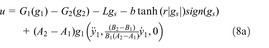
But, for the sake of simplicity, we are going to consider the case where the parameters of the drive and response systems are similar. Equation (8a) takes the simplified form in equation (8b) which is going to be used in the rest of the article

u = G_{1} (g_{1}) - G_{2} (g_{2}) - Lg - b \tanh (r | g |) sign (g)

(8b)

Equation (8) is designed to perform fast finite-time SMC with $(L, b, r) > (0, 0, 0)$ . As far as the jerk circuit is concerned, that controller is easy to implement in practice. In fact, the first two terms of equation (8) are automatically generated by the response circuit itself when the signal g is introduced. Replacing equations (5) and (7) in equation (8), the sliding surface and its time differential are, respectively, given by

s = - Lg

(9)

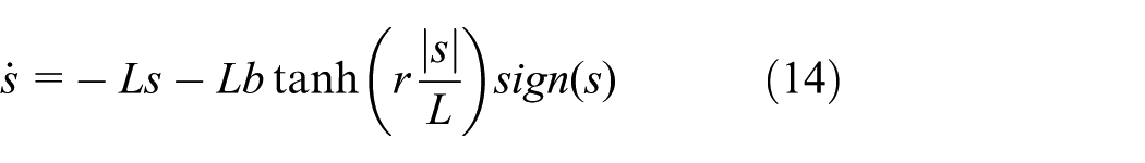
with the first derivative

\overset{\cdot}{s} = - L \overset{\cdot}{g}

(10)

Substituting equation (7) into equation (10) leads to

\overset{\cdot}{s} = - L (s - b \tanh (r | g |) sign (g))

(11)

According to equation (9)

| s | sign (s) = - L | g | sign (g)

(12)

so that

\tanh (r \frac{| s |}{L}) sign (s) = - \tanh (r | g |) sign (g)

(13)

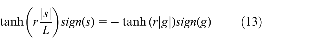
The substitution of equation (13) into equation (11) results in

\overset{\cdot}{s} = - Ls - Lb \tanh (r \frac{| s |}{L}) sign (s)

(14)

from where it can be deduced by multiplying both sides by s

s \overset{\cdot}{s} = - L s^{2} - bL | s | \tanh (r \frac{| s |}{L})

(15)

Considering the following Lyapunov function defined in equation (16) as

V = \frac{1}{2} s^{2}

(16)

equation (15) becomes

\overset{\cdot}{V} = - 2 LV - Lb \sqrt{| 2 V |} \tanh (r \frac{\sqrt{| 2 V |}}{L})

(17)

The direct integration of equation (17) being rather complex, it can however be approximated to obtain the expression of time at which the system state variables converge to the equilibrium point.

Using the change of variables defined in equation (18), equation (17) can now be transformed into a simpler expression depicted by equation (19)

V = r^{2} \frac{2 V}{L^{2}}, k = 2 L, q = 2 rb and a \leq \frac{1}{2} and a \leq \frac{1}{2}

(18)

\overset{\cdot}{V} = - kV - q \sqrt{V} \tanh (\sqrt{V})

(19)

The mathematical evidence of equation (20) is then used to bound equation (19) with the usual FTSM Lyapunov derivative in order to estimate the convergence time. Then, for all $V \in ℜ, - V^{a} \leq - \tanh (V)$ if and only if

0 < a \leq 1 and V \geq 0

(20)

After some mathematical manipulations of equations (19) and (20), we obtain

- kV - q V^{a + \frac{1}{2}} \leq - kV - q \sqrt{V} \tanh (\sqrt{V})

(21)

Supposing $(k', q') > (0, 0)$ and considering equation (20), additional conditions on $k'$ and $q'$ that verifies inequality in equation (22) below can be found

- k' V - q' V^{a} \geq - kV - q \sqrt{V} \tanh (\sqrt{V})

(22)

Applying the logarithm function on both sides of inequality in equation (22) leads to

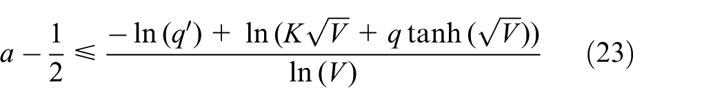
a - \frac{1}{2} \leq \frac{- \ln (q') + \ln (K \sqrt{V} + q \tanh (\sqrt{V}))}{\ln (V)}

(23)

with $K = (k - k')$ and $k'$ chosen to fulfil the condition $(k - k') > 0$ . Moreover, we have

\forall V \geq 0, \tanh (\sqrt{V}) \leq \sqrt{V}

(24)

Bounding equation (23) by equation (24) gives rise to the following relation

a - \frac{1}{2} \leq \frac{- \ln (q') + \ln (K \sqrt{V} + q \sqrt{V})}{\ln (V)}

(25)

In the simplified form, equation (25) is reduced to equation (26)

a \leq 1 + \frac{- \ln (q') + \ln (K + q)}{\ln (V)}

(26)

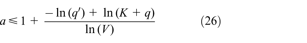
The above inequality (equation (26)) can be verified using its particular solution $q' = (K + q)$ . Therefore, the inequality in equation (22) is satisfied under the combined conditions $a \leq 1$ , $q' = (K + q)$ and $(k - k') > 0$ . At this point, it becomes obvious that it has been possible to bound the right-hand side of equation (19) by the usual FTSM Lyapunov function derivative which is easily integrable.

The next step is to estimate the synchronization time. Thus, equation (14) must fulfil the following conditions: $\overset{\cdot}{s} = f (s)$ and $f (0) = 0$ , with $s \in R$ . Having $V (s)$ defined positive in equation (16) and $a < 1$ , according to the definition of finite-time stability,^22,28,30 the equilibrium point $g = 0$ of the differential equation (7) is globally finite-time stable for any given initial condition $g (0) = g_{0}$ . Since g is a function with separable variables of the states of the system (position, velocity and acceleration), the system states and g will converge to 0 in finite time $T (g_{0})$ satisfying the following inequality

T_{1} (g_{0}) \leq T (g_{0}) \leq T_{2} (g_{0})

(27)

where

T_{1} (g_{0}) = \frac{2}{k (1 - 2 a)} \ln \frac{k V^{0.5 - a} (g_{0}) + q}{q}

(28)

and

T_{2} (g_{0}) = \frac{1}{k^{'} (1 - a)} \ln \frac{k^{'} V^{1 - a} (g_{0}) + q^{'}}{q^{'}}

(29)

are the corresponding finite times of the usual Lyapunov function derivative. The inequality in equation (27) is derived by integrating the relations in equations (21) and (22).

Remark 1

The unidirectional synchronization of two jerk systems that have different parameters can be done using the controller of equation (8b), but in this case only the variable g will be controlled. Meanwhile, with equation (8a), in addition to $g_{s}$ , the three state variables of the system are controlled and the synchronization times are then obtained by replacing g in equations (27)–(29) by $g_{s}$ . Indeed, for numerical computation with the fourth-order Runge–Kutta algorithm, the master and the slave are programmed using a system of three first-order differential equations which makes the time and computational memory space neither more, nor less important compared to those of the traditional methods. Using the system of third-order differential equations, the error states do not depend on the parameters of the master or slave system as is the case with the single first-order implicit equation.

Table 1 shows the initial conditions, the synchronization time and the system as well as the control parameter values that are used to synchronize two identical systems of equation (2) with different initial conditions.

Table 1.

Synchronization time of the error system with $G_{1} (g_{1}) = G_{2} (g_{2})$ , where x, y and z denote the velocity, position and acceleration, respectively.

Equations		(2a), (2d) and (2e)	(2b)	(2c)	(2f)	(2g)
Control values	b	0.1	5 × 10⁻⁶	5 × 10⁻⁶	5 × 10⁻⁶	5 × 10⁻⁶
	L	2	2	2	2	2
	r	1	1/3	1/3	1/3	1
Parameters’ values	A	0.6	0.6	0.6	0.25	0.0511
Parameters’ values	B	1	1	1	0.25	0.0073
drive initial conditions	x	0.1	0.1	0.1	0.1	0.1
	y	−5 × 10⁻⁷	−5 × 10⁻⁷	−5 × 10⁻⁷	−5 × 10⁻⁷	−5 × 10⁻⁷
	z	−1	−1	−0.1	−0.1	−1
Response initial conditions	x	10	10	−1	−1	10
	y	2	2	5	5	2
	z	10⁻⁴	10⁻⁴	−0.1	−0.1	10⁻⁴
$t_{d} (ms)$		1.2410	5.2195	5.2369	5.1623	4.7806

The last row of Table 1 displays values which confirm that the finite-time convergence was achieved. Each error system is obtained as $G_{1} (g_{1}) = G_{2} (g_{2})$ and the synchronization time calculated with $a = 0.9320$ and $k' ≲ k$ . In practice, one usually implements equation (2) using the nominal values of $1 K Ω$ and $0.1 μ F$ for resistors and capacitors, respectively.³ With these values, the fundamental frequency obtained is $f = 10^{4} / 2 π$ , and then the dimensionless time is $t = 2 π f \times t_{d}$ .

Figures 2 and 3 present the numerical results of equation (5) obtained with the controller in equation (8), using the values presented in Table 1 and considering equations (2a)–(2g), respectively. These figures show that the fast finite-time convergence is achieved for each error system and display their corresponding magnified images. It can be seen from Figures 4 and 5 that even at a precision of the order $10^{- 16}$ , the chattering phenomenon does not appear anymore. Moreover, the error values are closer to 0. These results confirm that our approach is more efficient compared to that used in Almeida et al.,¹¹ Genr et al.²⁸ and Suttirak and Pukdeboonn.²⁹ In systems (2a)–(2e), the nonlinear function is only a function of position which is not the case of systems (2f) and (2g). The results show that the use of an implicit variable remains valid for NFP, NFPV and NFPVA.

Figure 2.

Synchronization error variables versus dimensionless time t. Graphs on columns 1–5 represent the results for systems (2a)–(2e) of equation (2), respectively. Graphs from the top to bottom show in each column error on the variables x, y and z and the sliding variable g, respectively. Note that the precision here is of the order $10^{1}$ .

Figure 3.

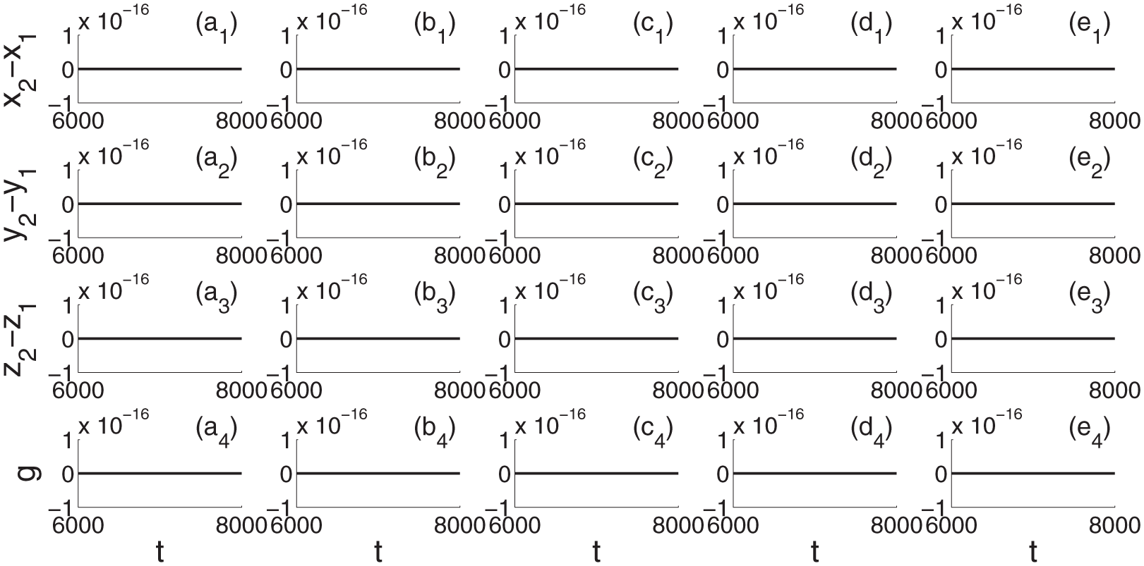
Synchronization error variables versus dimensionless time t. Graphs on columns 1 and 2 represent the results for systems (2f) and (2g) of equation (2), respectively. Graphs from the top to bottom show in each column the error on the variables x, y and $z,$ and the sliding variable g, respectively. Note that the precision here is still of the order $10^{1}$ .

Figure 4.

The closeness of synchronization error variables to the equilibrium point 0. Graphs on columns 1–5 represent the results for systems (2a)–(2e) of equation (2), respectively. Graphs from the top to bottom show in each column the error on the variables x, y and z and the sliding variable g, respectively. Note that the precision here is now of the order $10^{- 16}$ .

Figure 5.

The closeness of synchronization error variables to the equilibrium point 0 is reported. Graphs on columns 1 and 2 represent the results for systems (2f) and (2g) of equation (2), respectively. Graphs from the top to bottom show in each column the error on the variables x, y and $z,$ and the sliding variable g, respectively, with the precision of the order of $10^{- 16}$ .

The last row of Table 2 displays values which confirm that the finite-time convergence was achieved. Each error system is obtained as $G_{1} (g_{1}) \neq G_{2} (g_{2})$ and the synchronization time calculated with $a = 1 / 995$ . Systems (2a)–(2d) are chosen to be the response and system (2e) as the drive. These results improve those of Xu¹² where with two different systems only the asymptotic convergence could be obtained.

Table 2.

Synchronization time of error system with $G_{1} (g_{1}) \neq G_{2} (g_{2})$ , where x, y and z denote the velocity, position and acceleration respectively, and the indexes i and ii denote the response and drive systems, respectively.

Equations		(a)ⁱ	(b)ⁱ	(c)ⁱ	(d)ⁱ	(e)ⁱⁱ
Control values		$b = 60$ ; $L = 2$ ; $r = 1$
Parameters values		$A = 0.6$ ; $B = 1$
Initial conditions	x	10	10	−1	10	0.1
	y	2	2	5	2	−5 × 10⁻⁷
	z	10⁻⁴	10⁻⁴	−0.1	10⁻⁴	−1
$t (ms)$		$0.128$	$0.128$	$0.044$	$0.128$

Figure 6 presents the numerical results of equation (5) obtained with the controller of equation (8), the values in Table 2 and the response systems (2a)–(2d) of equation (2). Figure 8 presents the numerical results of equation (5) obtained using the controller of equation (8a), the values of Table 1 and systems (2f) and (2e) corresponding to the drive and response systems, respectively. The values of the controller used to plot the curves of Figure (8) are $b = 5 \times 10^{- 3}$ , $L = 0.07$ and $r = 1$ which give the synchronization time of $t = 11.3 ms$ . It confirms that the fast finite-time convergence is achieved for each error system. The magnification of those graphs displayed in Figures 7 and 8 shows that even if the chattering phenomenon does not disappear completely with a precision of the order $10^{- 15}$ , they are very close to 0. However, compared to the previous works^2,10,15,16 on a restricted class with the asymptotic active control method, the present results are still more accurate.

Figure 6.

Synchronization error variable versus dimensionless time t. Graphs on columns 1–4 represent the results for the drive system (2e) and the response system (2a)–(2d) of equation (2), respectively. Graphs from the top to bottom show in each column error on the variables x, y and z and the sliding variable g, respectively. The precision here is of the order $10^{1}$ .

Figure 7.

The closeness of synchronization error variable X to the equilibrium point 0. Graphs on columns 1–4 represent the results for the drive system (2e) and the response system (2a)–(2d) of equation (2), respectively. Graphs from the top to bottom show in each column error on the variables x, y and z and the sliding variable g, respectively. The precision here is of the order $10^{- 15}$ .

Figure 8.

Synchronization error variable versus dimensionless time t. Graphs (a)–(d) show the error on the variables x, y and z and the sliding variable g, respectively. Magnifications inside the boxes underline the occurrence of the chattering phenomenon at the precision of the order of $10^{- 14}$ .

Remark 2

A variation of the controller values affects the accuracy of the error and the synchronization time of the dynamical error system. When these values increase, the synchronization time decreases proportionally, while the accuracy deteriorates due to the increase of the chattering amplitude.

Experimental results

The laboratory experimental setup was designed using different values of components (Figure 9) for the drive and response circuits to obtain the results of Figure 10. In Figure 9, the diodes are of type 1N4148 and the resistors are worth $R = 1 k Ω$ . The direct current (DC) source voltage is $1.5 V$ , the capacitors are $10 nF$ , the variable resistor is adjusted at $2 k Ω$ and the op-amps are polarized at $\pm 12.5 V$ for the drive circuit. For the response circuit, the DC voltage source is fixed at $10.5 V$ , the capacitors are worth $20 nF$ , the variable resistor could take values from 1 to $27 k Ω$ and the op-amps are polarized at $\pm 9 V$ . Figure 11 shows the general form of the FTSM controller for this class of circuits. The output of the controller is connected to the response circuit by the negative pole of the voltage source V after its ground pin has been disconnected. For this particular case, the experimental values of $R_{i}$ ( $i = 1$ to 11) are as follows: $223 k Ω$ , $20.2 k Ω$ , $0.97 k Ω$ , $186 Ω$ , $4.1 k Ω$ , $0.97 k Ω$ , $497 Ω$ , $22 Ω$ , $1 k Ω$ , $1 k Ω$ and $83 k Ω$ . With a voltage summing amplifier, parts of the ypm and yppm signals are collected and added to the output of the controller before being injected into the response circuit. To be sure that all information from the error system remains part of the output of the controller, an op-amp of type LM318 is used because of its large frequency pass band. The response variable resistor (1–2.7 kΩ) and the DC voltage source (4.5–10.5 V) can also be varied to obtain the synchronized signals in Figure 12.

Figure 9.

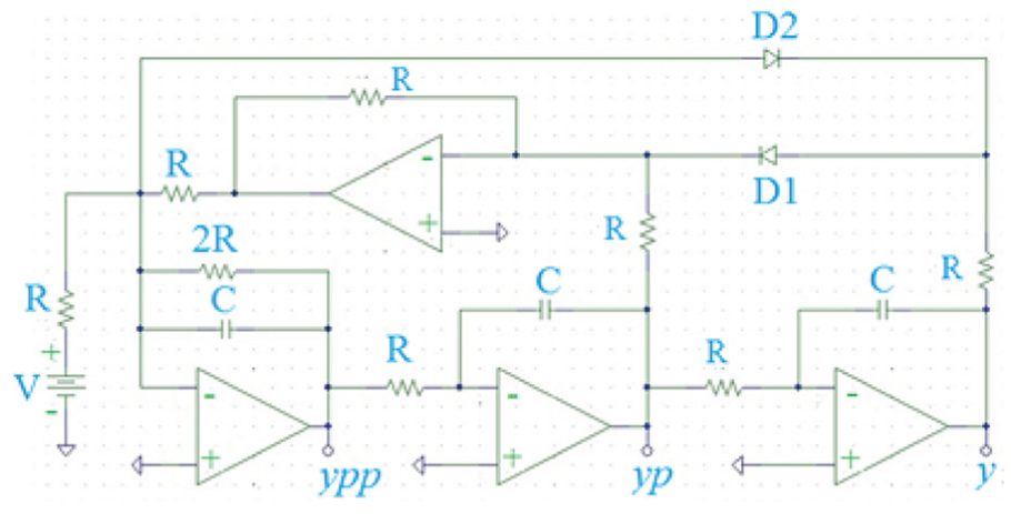
Chaotic circuit implementation of system (2a) of equation (2) using inverting op-amps (uA741). y, yp and ypp are the signals corresponding to the position, velocity and acceleration, respectively.

Figure 10.

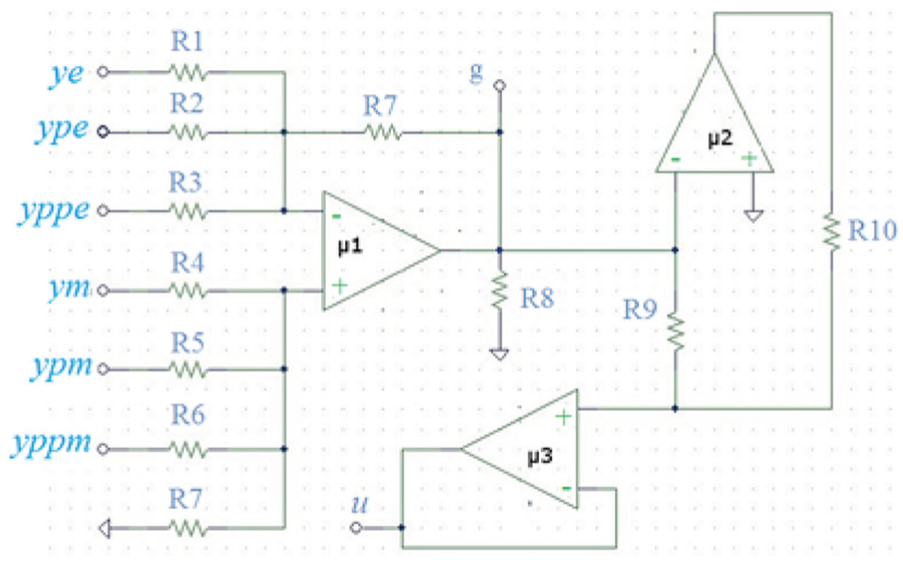
Experimental signals (a) $yp (1 V / div)$ , (b) $y (2 V / div)$ and (c) $ypp (2 V / div)$ at the input of the controller versus time $(2 μ s / div)$ . In each image, the signal (up) corresponds to the drive and the next (down) to the response circuits, respectively.

Figure 11.

Analogue circuit implementation of the controller using op-amps polarized at $\pm 12.5 V$ (µ1 = µ3 = TL072, µ2 = LM218). It should be noticed that each state of drive and response is collected by a follower (TL072 bias at $\pm 12.5 V$ ) before being injected into the controller. Indexes m and e refer to the drive and response signals, respectively.

Figure 12.

Experimental results of error signals from the controlled circuit: (a) signals ype versus ypm both measured at $0.5 V / div$ ; (b) signals ye versus ym both measured at $0.5 V / div$ ; and (c) signals yppe versus yppm both measured at $1 V / div$ .

Conclusion

In this article, the fast terminal time convergence is achieved for a class of jerk error systems with sigmoid nonlinear manifold. Few examples of systems with different types of parameters and nonlinearity are successfully synchronized for all state variables with the use of an implicit new variable with which third-order jerk dynamical equations could be transformed to a single first-order differential equation. A group of the Sprott circuits is also used for a practical device with good results to prove that the experimental setup of the proposed form of controllers can be designed using analogue components. It is then shown that the technique of using an implicit variable in the FTSM method can be generalized for any jerk circuits built with the same type of state components that has the form $\overset{\cdot\cdot}{y} + A \overset{\cdot\cdot}{y} + B \overset{\cdot}{y} = G$ independently of the form of the nonlinear function G. For any reason, temperature change for instance, electronic components can have their values affected. Such changes induce variation of the parameter values (A and B). As an outlook for this work, we aim at rendering the controller insensitive to such variations for better performance.

Footnotes

Handling Editor: Yueying Wang

Declaration of conflicting interests

The author(s) declared no potential conflicts of interest with respect to the research, authorship and/or publication of this article.

Funding

The author(s) received no financial support for the research, authorship and/or publication of this article.

ORCID iD

Tekou Nguazon

References

Eichhorn

Linz

Hänggi

Transformations of nonlinear dynamical systems to jerky motion and its application to minimal chaotic flows. Phys Rev E 1998; 58: 7151–7164.

Bai

E-W

Lonngren

Sprott

JC.

On the synchronization of a class of electronic circuits that exhibit chaos. Chaos Soliton Fract 2002; 13: 1515–1521.

Sprott

JC.

Simple chaotic systems and circuits. Am J Phys 2000; 8: 758–763.

Piper

Sprott

JC.

Simple autonomous chaotic circuits. IEEE T Circuits-II 2010; 57: 730–734.

Tchitnga

Nguazon

Louodop

et al . Chaos in a single op-amp–based jerk circuit: experiments and simulations. IEEE T Circuits-II 2016; 63: 239–243.

Tchitnga

Fotsin

Nana

et al . Hartley’s oscillator: the simplest chaotic two-component circuit. Chaos Soliton Fract 2012; 45: 306–313.

Kengne

Tsafack

Kengne

LK.

Dynamical analysis of a novel single opamp-based autonomous LC oscillator: antimonotonicity, chaos, and multiple attractors. Int J Dyn Control 2018; 6: 1543–1557.

Islam

Nikolov

Adaptive control and synchronization of Sprott J system with estimation of fully unknown parameters. J Theor Appl Mech 2015; 45: 45–58.

Shtessel

Edwards

Fridman

et al . Sliding mode control and observation (control engineering). New York: Springer Science + Business Media, 2013, pp.1–42.

10.

Louodop

Kountchou

Fotsin

et al . Practical finite-time synchronization of jerk systems: theory and experiment. Nonlinear Dynam 2014; 78: 597–607.

11.

Almeida

Alvarez

Barajas

JG.

Robust synchronization of Sprott circuits using sliding mode control. Chaos Soliton Fract 2006; 30: 11–18.

12.

Chaos synchronization between two different Sprott systems. Adv Theor Appl Mech 2010; 3: 195–201.

13.

Vaidyanathan

Output regulation of Sprott-I chaotic system by state feedback control. Int J Bioinform Biosci 2012; 2: 29–38.

14.

Song

Finite-time sliding mode control design for a class of uncertain conic nonlinear systems. IEEE/CAA J Automat Sin 2017; 4: 809–816.

15.

Daltzis

Volos

Nistazakis

et al . Analysis, synchronization and circuit design of a 4D hyperchaotic hyperjerk system. Computation 2018; 6: 1–19.

16.

Gonzalez Solis

Rosas Almeida

. Robust output synchronization of arrays of chaotic Sprott circuits. Adv Math Phys 2017; 2017: 1–9.

17.

Pietrala

Jaskuła

Bartoszewicz

. Terminal sliding mode control of second order systems with velocity constraint. In: Proceedings of the 19th international Carpathian control conference, Szilvásvárad, 28–31 May 2018, pp.223–227. New York: IEEE.

18.

Vaidyanathan

Sampath

Anti-synchronization of the hyperchaotic Lorenz systems by sliding mode control. IJCSE 2011; 3: 2450–2457.

19.

Wang

Shen

Karimi

et al . Dissipativity-based fuzzy integral sliding mode control of continuous-time T–S fuzzy systems. Int J Fuzzy Syst 2018; 26: 1174–1176.

20.

Slezák

Petržela

Evolutionary synthesis of cube root computational circuit using graph hybrid estimation of distribution algorithm. Audio Eng J 2014; 23: 549–558.

21.

Man

Fast terminal sliding-mode control design for nonlinear dynamical systems. IEEE T Circuits-I 2002; 49: 2261–2264.

22.

Yang

Finite-time terminal sliding mode tracking control for piezoelectric actuators. Abstr Appl Anal 2014; 2014: 1–9.

23.

Rhif

A high order sliding mode control with PID sliding surface: simulation on a torpedo. IJITCA 2012; 2: 1–13.

24.

Cheng

Park

Cao

et al . Quantized H∞ filtering for switched linear parameter-varying systems with sojourn probabilities and unreliable communication channels. Inform Sci 2018; 466: 289–302.

25.

Kao

Xie

Zhang

et al . A sliding mode approach to robust stabilisation of Markovian jump linear time-delay systems with generally incomplete transition rates. Nonlinear Anal Hybrid Syst 2015; 17: 70–80.

26.

Sprott

JC.

Elegant chaos: algebraically simple chaotic flows. Hackensack, NJ: World Scientific Publishing Co. Pte Ltd, 2010.

27.

Tchitnga

Zebaze Nanfa’a

Pelap

et al . A novel high-frequency interpretation of a general purpose op-amp-based negative resistance for chaotic vibrations in a simple a priori non chaotic circuit. J Vib Control 2016; 23: 744–751.

28.

Genr

Sheng

Liu

Finite-time sliding mode attitude control for a reentry vehicle with blended aerodynamic surfaces and a reaction control system. CJA 2014; 27: 964–976.

29.

Suttirak

Pukdeboonn

Finite-time convergent sliding mode controllers for robot manipulators. Appl Math Sci 2013; 7: 3141–3154.

30.

Hong

Huang

On an output feedback finite-time stabilization problem. IEEE T Autom Control 2001; 46: 305–309.

Simple finite-time sliding mode control approach for jerk systems

Abstract

Keywords

Introduction

Model equations

FTSM synchronization of two circuits encoded by an implicit equation

Remark 1

Remark 2

Experimental results

Conclusion

Footnotes

Declaration of conflicting interests

Funding

ORCID iD

References