Sage Journals: Discover world-class research

Abstract

This article presents a novel methodology for the inspection scheduling of gas turbine welded structures, based on reliability calculations and overhaul findings. The model was based on a probabilistic crack propagation analysis for welds in a plate and considered the uncertainty in material properties, defect inspection capabilities, weld geometry, and loads. It developed a specific stress intensity factor and an improved first-order reliability method. The proposed routine alleviated the computational cost of stochastic crack propagation analysis, with accuracy. It is useful to achieve an effective design for manufacturing, to develop structural health monitoring applications, and to adapt inspection schedules to airplane fleet experience.

Keywords

Damage tolerance reliability analysis crack detection fatigue probabilistic analysis

Introduction

Damage tolerance analysis methods have been used since the early 1970s to design and determine inspection intervals for aircrafts. Rogue flaws in structures will not grow to failure between scheduled inspections, based on the Paris–Erdogan¹ law. In 2001, the Federal Aviation Authority Advisory Circular (AC 33.14.1)² added a new damage tolerance element to existing design and life management processes for aircraft gas turbine rotors, based on the probabilistic fatigue analysis methodology that is implemented in the well-known DARWIN^® code by Wu et al.³ This procedure is used to predict uncontained engine failure because of microcracks and micropores that are caused by alpha-phase anomalies in titanium alloys. Structural health monitoring technologies allow for the detection of structural damage with crack growth damage during component lifecycles by means of sensors. These techniques have developed rapidly over the last two decades, which has enabled the implementation of component operating conditions into crack growth models, as explained by Coppe et al.⁴

Welded structural components may contain defects that do not represent nominal conditions. If undetected, they can lead to unexpected failure of the engine and unscheduled component replacement. Kale and Haftka,⁵ Opgenoord and Willcox,⁶ and Millwater and Wieland⁷ developed probabilistic frameworks to predict the risk of fracture associated with undetected weld defects and to define the proposed inspections plans. These methods consider the sensitivity of manufacturing conditions, inspection methods, and component-loading conditions to achieve reliability target with minimum inspection and manufacturing costs.

In this article, we present a new probabilistic fatigue analysis methodology for gas turbine welded structures, which is similar to those reported in the literature,^3,5,7,8 but with several substantial differences. It uses an improved first-order reliability method (FORM) which includes fracture variability to evaluate the component reliability as was done by Madsen et al.,⁹ Kale and Haftka,⁵ and Feng et al.,^10,11 and to estimate the crack size distribution after inspection. In this sense, the new methodology is more efficient. Furthermore, it updates damage growth parameters based on the data obtained from inspections as done by Kapur and Lamberson,¹² Coppe et al.,⁴ Kim et al.,¹³ and Bhachu et al.,¹⁴ which allows for an update of the inspection plan. The crack growth law incorporates an “ad hoc” stress intensity factor (SIF) formulation for welds,¹⁵ which is defined by elementary functions that are obtained by solving the integral of the Paris–Erdogan equations for a surface crack in a welded plate. Thus, inspection scheduling can be planned based on the reliability updating of gas turbine welded structures using this new efficient methodology. The flowchart in Figure 1, explained by Opgenoord and Willcox,⁶ shows the different steps in the methodology. It has four loops that can be repeated separately or simultaneously (all loops at the same time) during all of the component life phases.

Figure 1.

Schematic of the proposed process for component inspection definition.

The first loop, which is typically used in the component design process, defines the inspection based on target reliability. As a first step, the target reliability is established and the welding parameters are defined (explained in section “Inputs: target reliability and welding parameters”). The defect growth laws are established as described in section “Crack growth model.” A reliability evaluation is carried out as explained in sections “Fracture limit state function,”“Fatigue limit state function,” and “Fracture probability: FORM + fracture.” A comparison of this result with the required reliability yields a first inspection schedule.

The second loop, which is typically used in the manufacturing definition process, is a sensitivity analysis to estimate the impact of and identify the most critical welding parameters. The welding parameters are used as the input data together with the defect growth law, to evaluate the reliability, and a parameter sensitivity study is performed as described in section “Loop 2: sensitivity of welding parameters.” The results and consideration of the inspection and manufacturing methods allow for the definition of a new set of welding parameters. The new parameters can be used as the feedback to the first loop to define a new inspection schedule.

The third loop corresponds to the forecasting of reliability evaluation after an inspection. The welding parameters are used as the input data and, with the defect growth law, the defect size and rate that are found during inspection are forecast as explained in section “Loop 3: reliability evaluation after inspection.” The reliability evaluation is updated based on the inspection, which provides a typical saw-tooth reliability graph.

The fourth loop corresponds to the service support process. In addition to the steps in the third loop, the defect size that is estimated in loop 3 is compared with the inspection findings (section “Loop 4: probabilistic damage growth model update by inspection findings”). Thus, using the likelihood analysis as suggested in López de Lacalle et al.,¹⁶ the welding parameters can be updated, and loops 1, 2, and/or 3 can be rerun to obtain an “Inspection scheduling based on reliability updating.”

As outlined in the previous paragraphs, based on the flowchart in Figure 1, the article is structured as follows. Sections “Loop 1: reliability evaluation and first inspection schedule” and “Loop 2: sensitivity of welding parameters” contain the damage growth model parameters, the crack growth model, and the novel FORM + fracture reliability evaluation methodology. Section “Loop 3: reliability evaluation after inspection” describes the procedure to evaluate and update the reliability after an inspection. Section “Loop 4: probabilistic damage growth model update by inspection findings” explains the methodology to forecast inspection findings and the maximum-likelihood estimator (MLE) methodology to update the crack growth model used. Section “Numerical example: application to gas turbine engine components” presents, for illustrative purposes, a numerical example of an electron beam weld in a pressure containment case and discusses the performance of the method. Section “Conclusion” presents the main conclusions of the work.

Loop 1: reliability evaluation and first inspection schedule

Inputs: target reliability and welding parameters

After defining the target reliability requirement (failure probability in N load cycles), the welding parameters (weld fatigue crack growth variables) must be introduced as the input data and considered as statistical variables.¹⁷ The welded structural components under study are divided into different areas with the same failure probability.¹⁸ Each area has its own set of parameters listed in Table 1, and the impact on fatigue growth is evaluated individually depending on the welding process and its load. Most parameters are considered statistical variables with the corresponding mean and standard deviations of a probability distribution function (PDF) that is intentionally “right tailored adjusted” to a normal or lognormal distribution. The parameters are grouped in different categories depending on their nature, as shown in Table 1.

Table 1.

Welding parameters.

Parameter group	Parameter	Unit	Description
Inspections	a_i	mm	Half of a surface anomaly initial size
	a_f	mm	Half of a surface anomaly size that triggers component fracture
	δ	mm⁻¹	Crack occurrences per unit weld length
Material properties	n	–	Paris–Erdogan equation constants
	c	(mm/cycle)/(MPaⁿ m^−n/2)	Paris–Erdogan equation constants
	K_Ic	MPa m^1/2	Material fracture toughness
Welding geometry and acceptance criteria	υ	–	Constant to define the SIF for welds
	t_w	mm	Butt weld real thickness
	e	–	Weld linear misalignment expressed as the percentage of thickness
	α	rad	Weld angular misalignment
Loads and FEM	σa	MPa	Axial mean stress
	σb	MPa	Bending surface stress
	N	–	Number of load cycles
Method uncertainty	λ_w	–	Surface crack stress correction factor for thickness
Method uncertainty	Θ	–	Surface crack stress correction factor for elliptical integral

SIF: stress intensity factor; FEM: finite element model.

Inspections

The initial defect size a_i (prior to the part’s first usage) PDF is obtained from the probability of detection (POD) curves of several nondestructive tests (NDTs), which are applied to the component during the manufacturing processes, namely, X-rays, fluid penetrant inspection, eddy current, and ultrasonic inspection. Thus, the POD curves are defined in the industrial NDT standards, after a statistical hit–miss analysis of a test piece inspection finding.¹⁹

The manufacturing crack occurrences per unit weld length δ are evaluated based on the number of welding areas of the reworked part and consideration of the POD curve. δ is considered a constant parameter, because it is proportional to the failure probability to be evaluated, and it is not considered in the crack propagation analysis. The final surface crack size a_f prior to fracture is correlated fully with the fracture toughness statistical variable K_Ic, which is one of the material properties that is specified in the following section.

Material properties

The weld defects are considered sharp cracks that grow according to fatigue growth rates defined by the Paris–Erdogan parameters c and n.¹ The parameter c is considered a statistical variable, whereas the parameter n is a constant to ease integration of the Paris–Erdogan equation. Failure occurs because fracturing occurs when the defect size reaches the fracture toughness K_Ic, with a specific final crack size a_f.^20,21 The fracture test specimen thickness needs to represent the plane stress/strain working condition of the structural member under study. The proposed methodology assumes that the weld residual stresses are negligible.²² In addition, the advantages of the crack growth threshold and retardation effects on the fatigue crack growth are not considered.

Welding geometry and acceptance criteria

The butt welds’ acceptance criteria²³ restrict the four welding geometry statistical variables in Figure 2, namely, the resultant angular misalignment (α), the weld linear misalignment after welding the joining sheets (e), the weld thickness variation related to the welding parts’ nominal thickness (t_w),¹⁸ and the resultant stress concentration factor of the weld crown–root geometry (υ). The welding process is unacceptable until these variables are below specified limits. Each variable has an independent PDF, with a mean value that corresponds to the component’s nominal condition, and standard deviations that agree with the welding acceptance limits.

Figure 2.

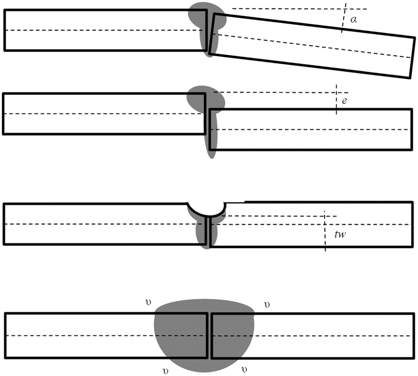
Welding geometry variables.

Loads and the finite element method

Because of manufacturing limitations and simplifications in the welding process, butt welds are produced in the location with the lowest component thickness. The stress behavior of the parts corresponds to a shell element, and the load is defined by two independent statistical variables that are obtained from an uncracked finite element model (FEM), namely, the axial stress σa and the bending stress σb. Both variables are considered to be uncorrelated such that the thermal and mechanical loads are considered independently. The loads are repeated N times (which is a constant value that is defined in the specifications) during the welded component life.

Method uncertainty

In most cases, it is impossible to model three-dimensional (3D) crack growth in a cracked FEM. Instead, the proposed methodology uses an analytical SIF,^24,25 by considering the stress history obtained using an uncracked FE model. The main simplifying assumptions are that crack growth occurs within a plane and that the aspect ratio of the crack remains constant during the growth process.²⁶ The bivariant stresses²⁷ and thermal load relaxation when the crack opens^28,29 are not considered.

The statistical variables λ_w and Θ represent the variation in SIF between the most realistic crack growths based on a 3D cracked FEM and the simple proposed analytical model. Thus, the method uncertainty PDF variables measure the conservatism and possible improvement if a more realistic model is used. The PDF mean value corresponds to the nominal analytical SIF values, and the PDF standard deviation corresponds to the differences between the nominal analytical and the accurate 3D FEM model crack growth values.

Method: probabilistic damage growth model

Crack growth model

This article uses the original Paris–Erdogan model¹ to predict growth anomalies in butt welds. The parameters c and n were estimated experimentally for the material using a log–log scale plot to relate the growth rate da/dN to the SIF ΔK as shown in equation (1)

\frac{da}{dN} = c {(Δ K)}^{n}

(1)

For the SIF, a mode I propagation law of a surface elliptical crack in a plate was considered. The formulation by Wilson²⁴ and Newman and Raju²⁵ was used, which calculates the SIF as a function of the axial load σa and bending load σb in equation (2). The constant Θ corresponds to the surface crack stress correction factor for an elliptical integral, and λ_w, λ_t, and λ_b correspond to the tabulated surface crack stress correction factors for thickness, axial loading, and bending loading, respectively

Δ K = \frac{λ_{ω}}{Θ} (λ_{t} \cdot σ a + λ_{b} \cdot σ b) \sqrt{π \cdot a}

(2)

Two SIFs could be considered: one in the surface of the crack and the other in the deepest point of the surface crack at 90°. Butt welds work mainly under bending load, so the crack grows in the weld surface, and therefore the SIF corresponds to the welded surface. During crack growth, a constant relationship of 0.563 is considered between the crack depth and the crack length (size) on the surface according to Sundararajan and Hudak²⁶ for equation (2). Consequently, equation (2) becomes equation (3), which depends on the crack size a, weld thickness t, axial stress σa, and bending stress σb

Δ K = \frac{1}{1.57} ((1.119 + 0.431 \frac{a}{t}) σ a + 1.076 \cdot σ b) \sqrt{π \cdot a}

(3)

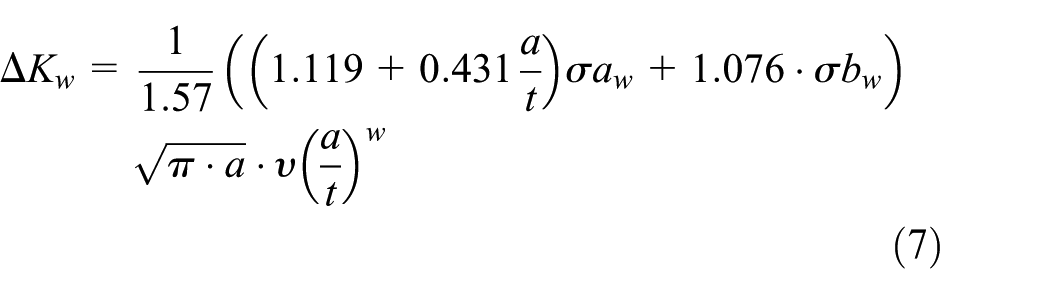
Here, ΔK, σa, and σb in equation (3) must be adapted to consider butt weld geometrical effects, which become ΔK_w, σa_w, and σb_w, respectively, in equation (7), and which represent the propagation law of a surface elliptical crack in a welded plate. First, the weld thickness t_w is updated for the axial and bending stresses in equations (4) and (5), respectively.²³ Weld manufacturing misalignment e and angularity α increase the bending stress²³ as shown in equation (5). Finally, the power-law function of equation (6) defines the stress concentration in the weld crown and root,³⁰ which yield equation (7)

σ a_{w} = σ a (\frac{t_{w}}{t})

(4)

σ b_{w} = {(\frac{t_{w}}{t})}^{2} (σ b + σ a (\frac{t_{w}}{t}) (3 e + \frac{3 \cdot α \cdot ll}{2 t}))

(5)

Δ K_{w} = Δ K \sqrt{π \cdot a} \cdot υ {(\frac{a}{t})}^{w}

(6)

\begin{matrix} Δ K_{w} = \frac{1}{1.57} ((1.119 + 0.431 \frac{a}{t}) σ a_{w} + 1.076 \cdot σ b_{w}) \\ \sqrt{π \cdot a} \cdot υ {(\frac{a}{t})}^{w} \end{matrix}

(7)

Fracture limit state function

For an evaluation of the reliability, the fracture and fatigue limit state functions³¹ are defined in sections “Fracture limit state function” and “Fatigue limit state function,” respectively, according to Figure 1. Then, the fracture probability is evaluated in section “Fracture probability: FORM + fracture,” as shown in Figure 1.

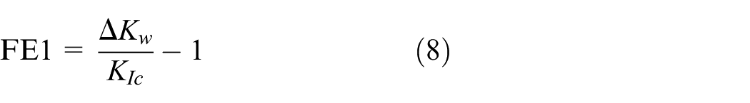
With regard to the fracture limit state function, in a structure, the crack grows until the material fracture toughness K_Ic is reached. If the crack section material works in the plastic region, the fracture toughness needs to be corrected.¹⁵ The fracture of the crack section occurs when the state function FE1 defined in equation (8) becomes 0, starting from −1 when the crack size is small

FE 1 = \frac{Δ K_{w}}{K_{Ic}} - 1

(8)

Fatigue limit state function

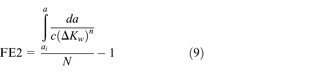
A second state function FE2 is established in equation (9), which relates the crack growth in a period for a number of load cycles N. The function is obtained by substituting equations (4)–(6) into equation (9). FE2 becomes 0 when, at N cycles, the crack size is a, whereas it is −1 when the crack growth is slow. Both state functions need to become 0 to fracture at N load cycles. FE2 and FE1 must be 0 and negative, respectively, to achieve a specific crack size a in N load cycles during crack growth

FE 2 = \frac{\int_{a_{i}}^{a} \frac{da}{c {(Δ K_{w})}^{n}}}{N} - 1

(9)

The integral in equation (9) is a binomial integral type, developed in equation (10), where c₀ and c₁ are the intermediate variables to simplify the expression, with the values shown in equations (11) and (12), respectively. The integral is solved using elementary functions through the variable change c₀ + c₁a = t^s because the binomial integration requirements are fulfilled:³²n is a fraction and −(w + 1/2)n is an integer

\int_{a_{i}}^{a} \frac{da}{c {(Δ K_{w})}^{n}} = \int_{a_{i}}^{a} a^{- (w + \frac{1}{2}) n} {(c_{0} + c_{1} \cdot a)}^{- n} da

(10)

c_{o} = \frac{c^{\frac{1}{n}}}{1.57} υ {(\frac{1}{t})}^{w} (1.119 \cdot σ a_{w} + 1.076 \cdot σ b_{w})

(11)

c_{1} = \frac{c^{\frac{1}{n}}}{1.57} υ {(\frac{1}{t})}^{w} ((\frac{0.431}{t}) σ a_{w})

(12)

Fracture probability: FORM + fracture

The probability of failure Pf_w after N load cycles in equation (13) is calculated as follows. First, the structure welds are divided into different areas with the same fracture risk. Each area of length is selected with a constant crack growth rate that is proportional to the weld length multiplied by the maximum area stress power to the Paris constant n. The event failure of each area, F_i, is evaluated individually and each zone has a defect occurrence probability per unit of length δ. If the occurrence rate of the defects is small, the probability of having two or more defects in the same part is negligible and the failure probability is the sum of the failure probability of the individual areas.^3,33 Thus, the overall risk probability is the union of the na individual areas’ failure, and if the failure probability of each area is small, the expression can be approached as the addition of all individual probabilities^3,33

P f_{w} (N) = P (F_{1} \cup F_{2} \cup \dots \cup F_{na}) \approx \sum_{i = 1}^{na} P f_{Fi} (F_{i})

(13)

Conventional FORM^34–36 calculation uses the FE2 = 0 state equation. Because of the large variability in fracture toughness in the welds, K_Ic is considered a variable in this work, so the FORM calculation needs to incorporate an additional constraint FE1 = 0 in equation (14) to update the critical crack size a_f between the design most probable point (DMPP) and the failure most probable point (FMPP). This approach will be referred to as “FORM + fracture.” The FMPP is obtained at the minimum measured distance between the DMPP and the failure surface. A nonlinear optimization problem with one constraint (FE1 = 0) is solved using the method of feasible directions.³⁷ During the optimization process, the critical crack size parameter a_f is updated to fulfill failure mode FE2 = 0 and restrict FE1 = 0 in the FMPP. By means of an iterative algorithm, a reliability index β_fi (equation (15))^34–36 which represents the minimum distance between the DMPP and the FMPP in a normalized space (see Figure 3) is obtained. This minimum distance corresponds to the number of standard deviation distances between the FMPP and the DMPP

\begin{matrix} P f_{w} (N) \approx \sum_{i = 1}^{na} P f_{Fi} (F_{i}) \\ = \sum_{i = 1}^{na} L a_{i} \cdot δ \cdot P (FE 2_{i} (N, a) ⩾ 0 & FE 1_{i} (a) = 0) \\ = \sum_{i = 1}^{na} L a_{i} \cdot δ \cdot Φ (- β_{Fi}) \end{matrix}

(14)

β_{fi} = min \sqrt{{(x - μ)}^{T} C^{- 1} (x - μ)}

(15)

Figure 3.

FORM + fracture methodology.

The reliability index β_fi evaluated at different load cycles N establishes the failure probability Pf_w (equation (16)) and defines the first inspection interval to guarantee the target component reliability, which is the objective of loop 1 in Figure 1 as described in the section “Introduction.” When the failure probability reaches the failure target value, an inspection to remove the defective parts is needed

P f_{w} (N) \approx \sum_{i = 1}^{na} La \cdot δ \cdot Φ (- β_{Fi})

(16)

Loop 2: sensitivity of welding parameters

Once the reliability index β has been evaluated to determine the first inspection interval in loop 1 (see Figure 1), loop 2 performs a sensitivity study of welding parameters to identify the most critical parameters. The reliability sensitivity to the mean and standard deviation of the input variables are expressed as functions of the reliability index β. The vector that joins DMPP and FMPP in the same normalized space determines the gradient vector α_i, which approximates the sensitivity of the mean and standard deviation values of all variables related to the input variables (equations (17) and (18))^38,39

\frac{\partial β_{fi}}{\partial μ_{j}} \approx α_{j}

(17)

\frac{\partial β_{fi}}{\partial σ_{j}} \approx - β \cdot α_{j}^{2}

(18)

By means of these equations, the input variable mean and standard deviation relevance in the reliability are calculated, and road maps to improve the welded component reliability can be defined.

Loop 3: reliability evaluation after inspection

Once the reliability index β has been evaluated to determine the first inspection interval in loop 1 (see Figure 1), loop 3 forecasts a defect size and rate that will be found during the inspection.

Defect size forecasting

The probability of a failure decreases after each inspection because, whenever cracks are detected, the components are either rejected or repaired. Two inputs are necessary to establish the number of cracks that will be detected during an inspection, namely, the component crack size distribution at inspection and the POD of the selected inspection method.¹⁹

To evaluate the crack size PDF after N load cycles, the FORM optimization loop is used^34–36 and a Monte-Carlo simulation (MCS) is avoided. Thus, the fracture toughness PDF (FE1) does not take part in the defect growth calculation, and the FORM calculation only incorporates FE2 = 0. Equation (19) repeats the FORM optimization loop at each area, sweeping different defect sizes, as illustrated in Figure 4

\begin{matrix} P (N, a) \approx \sum_{i = 1}^{na} P_{i} (N, a) = \sum_{i = 1}^{na} L a_{i} \cdot δ \cdot P (FE 2 (N, a) ⩾ 0) \\ = \sum_{i = 1}^{na} L a_{i} \cdot δ \cdot Φ (- β_{a}) \end{matrix}

(19)

Figure 4.

FORM to predict finding sizes.

The analysis is a sweep across different defect inspection sizes. At each size, the crack distribution probability Pi(N,a) is obtained by an iterative algorithm. β_a represents the probability of having a defect size larger than a; and represents the minimum distance between the DMPP and the defect size most probable point (DSMPP) in a normalized space, as shown in Figure 4. The unconstrained nonlinear optimization problem is solved using the method of feasible directions.³⁷

Defect rate forecasting

The PDF of the crack size that will be detected during the inspection a is obtained by the concurrence of three circumstances: the crack existence Pi(N,a), the crack detection POD(a), and the crack occurrence δ. The detected crack rate per length unit in each zone δ_di is obtained by integrating these three factors for all crack sizes (equation (20))³

δ_{di} = \int_{0}^{\infty} δ \cdot P (FE 2_{i} (a_{d}) = 0) \cdot POD (a_{d}) da

(20)

Equation (21) provides the percentage of defective part removal δ_dpr, calculated as the mean value of the crack rate detected per unit of length δ_di

δ_{drp} = \frac{\sum_{i = 1}^{na} δ_{di} \cdot L a_{i}}{\sum_{i = 1}^{na} L a_{i}}

(21)

Fracture probability and inspection plan

The fracture probability obtained in section “Method: probabilistic damage growth model” is updated based on the defect rate forecasting. Once again, the reliability index β_fi establishes the failure probability Pf_w (equation (15)) and defines the inspection interval to guarantee the target component reliability. After the inspection, cracked elements are removed or repaired, and the component reliability is kept on target until the next inspection. When the failure probability reaches the failure target value, an inspection to remove the defective parts is needed. The removal of these defective parts reduces the failure probability a δ_dpr percentage (equation (22)). The results provide a typical saw-tooth graph that maintains the failure probability above the target³

P f_{w} (N) \approx (1 - δ_{dpr}) \sum_{i = 1}^{na} La \cdot δ \cdot Φ (- β_{Fi})

(22)

As a result, loop 3 updates the reliability evaluation based on the prediction of the number and size of defects that occur in each inspection.

Loop 4: probabilistic damage growth model update by inspection findings

Once the reliability index β has been evaluated to determine the first inspection interval in loop 1 (see Figure 1), and this reliability evaluation has been updated in loop 3, loop 4 compares the defect size forecast in loop 3 with real inspection findings.

The number of inspection findings will differ from the value forecast by equation (19); thus, the difference is used to tune the detected crack rate per length unit δ. For such purposes, an exponential distribution is commonly used.⁴⁰

The size of the component inspection findings redefines the inspection plan. Two different approaches were evaluated in this work: the MLE, which is similar to the Bayesian approach,^12,13 and the failure-weighted mean square value (FWMSV).

The MLE is used to update the mean and standard deviations of the variables in Table 1. The process optimizes the cycle, the objective of which is to maximize the likelihood of the sum of probabilities for the nf defects found during the inspection (equation (23)). The optimization loop includes defect size forecasting calculations described in section “Loop 3: reliability evaluation after inspection” for each defect found, using the method of feasible directions³⁷

MLE = \sum_{i = 1}^{nf} \frac{P (a_{i}, N_{i})}{nf}

(23)

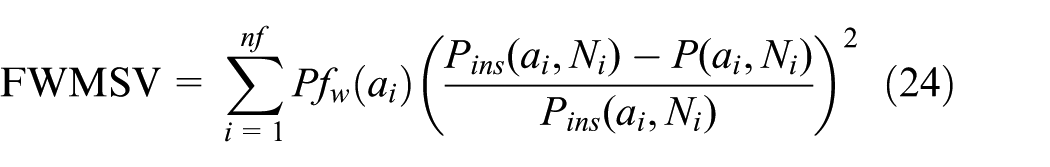
The FWMSV is used to update the mean and standard deviations of the variables in Table 1. In this case, the process optimizes the cycle, the objective of which is to minimize the mean square difference of the crack size exceedance probability weight by the failure probability when that crack size is detected (equation (24)). Again, the optimization loop includes defect size forecasting calculations in section “Loop 3: reliability evaluation after inspection” for each defect found, using the method of feasible directions,³⁷ together with fracture probability calculations similar to that presented in section “Fracture probability: FORM + fracture” but using the defect size as the initial crack size a_i

FWMSV = \sum_{i = 1}^{nf} P f_{w} (a_{i}) {(\frac{P_{ins} (a_{i}, N_{i}) - P (a_{i}, N_{i})}{P_{ins} (a_{i}, N_{i})})}^{2}

(24)

In both cases, the parameter update is guided and limited by the uncertainty weight that is applied to each variable. Those uncertainty weights modify the parameter gradient used during the optimization loop and avoid inconsistent solutions. They are selected by engineering judgment and are based on the confidence levels of the parameters in Table 1.

After the original parameters in Table 1 are updated to reach the maximum MLE or the minimum FWMSV, loops 1, 2, and/or 3 can be rerun to obtain an “Inspection scheduling based on reliability updating” as suggested by López de Lacalle et al.¹⁶

Numerical example: application to gas turbine engine components

This section presents a numerical example to evaluate the reliability of a welded jet engine case based on the developed methodology. The geometry in Figure 5 corresponds to a circular butt electron beam weld that axially joins two cylinders of 2.2 mm thickness and 707 mm diameter of a nickel-based heat-resistant alloy. The loads are caused by the temperature difference between the jet engine core and the ambient atmosphere during a flight cycle. Each flight corresponds to a single load cycle, which starts and ends with a null load and reaches the maximum stress level at take-off. Skin loads are applied in 36 mm lengths, with 100 MPa outside and 60 MPa inside the cylinder, following a parabolic stress distribution in the circumferential direction (see Figure 6).

Figure 5.

Jet engine welded case.

Figure 6.

Circumferential maximum skin stress distribution (MPa).

Table 2 summarizes the mean value and standard deviation of the parameters considered in the calculation, as presented in Table 1. The manufacturing crack occurrence per unit weld length δ is 5.0 × 10⁻⁵. The butt weld acceptance criterion restricts the standard deviation of the misalignment to 5%, the thickness reduction to 3%, the angular misalignment to 0.05 rad, and the stress concentration factor variability to 15%. The defect POD has a mean size of 0.38 mm with a 1.04 mm standard deviation.⁴¹

Table 2.

Parameters considered in the example.

Parameter group	Parameter	Unit	Mean value	Standard deviation	Probability distribution function
Inspections	a_i	mm	Ln(0.38)	0.677	Lognormal
	a_f	mm	2.83	–	–
	δ	mm⁻¹	5.0 × 10⁻⁵	–	–
Material properties	n	–	3.5	–	–
	c	(mm/cycle)/(MPaⁿ m^−n/2)	85.4 10⁻⁷	4.27 × 10⁻⁷ (5%)	Lognormal
	K_Ic	MPa m^1/2	8.125	0.52 (5.5%)	Normal
Welding geometry and acceptance criteria	ν	–	1.086	0.18 (16.7%)	Normal
	t_w	mm	0	0.06 (3%)	Normal
	e	–	0	0.11 (5%)	Normal
	α	rad	0	0.0583	Normal
Loads and FEM	σa	MPa	20	2 (10%)	Normal
	σb	MPa	80	8 (10%)	Normal
	N	–	300	–	–
Method uncertainty	λ_w	–	1.076	0.108 (10%)	Normal
Method uncertainty	Θ	–	1.429	0.14 (10%)	Normal

FEM: finite element model.

The Paris constant n has a value of 3.5, whereas c incorporates the defect growth variability. The fracture toughness K_Ic considers the variability of the final crack size before fracture. As discussed in section “Inputs: target reliability and welding parameters,” the effect of weld residual stresses,²² the crack growth threshold, and the retardation effects are not considered in the fatigue crack growth.

The weld reliability target needs to be below 1.4 × 10⁻⁴ during 300 load cycles, to fulfill component requirements. A deterministic crack propagation analysis, which considers the existence of a crack in the most stressed location at the beginning of the component life and the mean value of the parameters in Table 2, predicts a structural failure at 530 load cycles.

Loop 1: probabilistic damage tolerance assessment

The method in section “Loop 1: reliability evaluation and first inspection schedule” allows for a definition of the inspection based on the target reliability. As a first step, the target reliability is established and welding parameters are defined, as explained in section “Inputs: target reliability and welding parameters.” Next, the defect growth laws are established as described in section “Crack growth model” and the reliability evaluation is carried out as explained in sections “Fracture limit state function,”“Fatigue limit state function,” and “Fracture probability: FORM + fracture.” Finally, this result is compared with the required reliability, and a first inspection schedule is established.

The unique welding process is divided into different areas. Each area of length is selected to have a constant crack growth rate that is proportional to the weld length multiplied by the maximum area stress power to the Paris constant n, as explained in section “Fracture probability: FORM + fracture.” Each area is evaluated independently with its own set of parameters and its own probability failure.

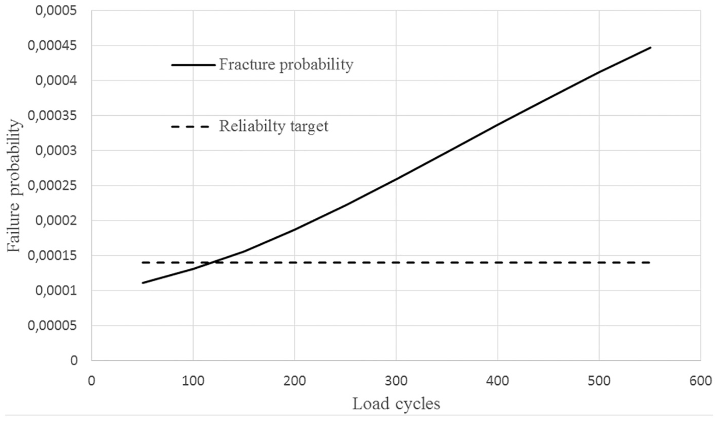
The weld division process and the failure analysis explained above are repeated, until the overall weld probability (equation (13)) converges. Table 3 shows the results with 12 areas at 300 load cycles, and the calculations are repeated at different load cycles to build a fracture probability curve shown in Figure 7.

Table 3.

Failure probability at 300 cycles and the end of the component service life.

Area	Stress (MPa)	Axial position star (mm)	Axial position end (mm)	Equivalent length (mm)	Reliability index	Crack probability per unit of length	Fracture probability	Area failure probability	Maximum error (%)
a	100.0	0	1	2	0.5274	5.00 × 10⁻⁵	2.99 × 10⁻¹	2.99 × 10⁻⁵	0.1
b	99.7	1	2	2	0.5395	5.00 × 10⁻⁵	2.95 × 10⁻¹	2.95 × 10⁻⁵	0.2
c	98.8	2	2.5	1	0.5756	5.00 × 10⁻⁵	2.82 × 10⁻¹	1.41 × 10⁻⁵	0.1
d	98.1	2.5	3	1	0.6036	5.00 × 10⁻⁵	2.73 × 10⁻¹	1.37 × 10⁻⁵	0.1
e	97.2	3	3.5	1	0.6393	5.00 × 10⁻⁵	2.61 × 10⁻¹	1.31 × 10⁻⁵	0.1
f	96.2	3.5	4	1	0.6787	5.00 × 10⁻⁵	2.49 × 10⁻¹	1.24 × 10⁻⁵	0.1
g	95.1	4	4.5	1	0.7216	5.00 × 10⁻⁵	2.35 × 10⁻¹	1.18 × 10⁻⁵	0.1
h	93.8	4.5	5	1	0.7717	5.00 × 10⁻⁵	2.20 × 10⁻¹	1.10 × 10⁻⁵	0.2
i	92.3	5	5.5	1	0.8287	5.00 × 10⁻⁵	2.04 × 10⁻¹	1.02 × 10⁻⁵	0.2
j	90.7	5.5	6	1	0.8884	5.00 × 10⁻⁵	1.87 × 10⁻¹	9.36 × 10⁻⁶	0.2
k	88.9	6	7	2	0.9542	5.00 × 10⁻⁵	1.70 × 10⁻¹	1.70 × 10⁻⁵	0.6
l	84.9	7	10	6	1.0951	5.00 × 10⁻⁵	1.37 × 10⁻¹	4.10 × 10⁻⁵	4.6
m	69.1	10	18	16	1.5732	5.00 × 10⁻⁵	5.78 × 10⁻¹	4.63 × 10⁻⁵	8.9
Weld	100.0	N/A	N/A	17.34	0.5274	5.00 × 10⁻⁵	2.99 × 10⁻¹	2.59 × 10⁻⁴	15.5

N/A: not available.

Figure 7.

Failure probability without inspection.

The calculations to obtain the fracture probability (section “Method: probabilistic damage growth model”) are repeated for different load cycles, which gives the failure probability curve in Figure 7. The failure probability reaches the failure target value, close to a hundred load cycles, and an inspection is necessary to remove or repair the defective parts.

Loop 2: weld parameter sensitivity

The method in section “Loop 2: sensitivity of welding parameters” allows us to obtain the input parameter sensitivity and an identification of the main variables that contribute to failure probability. The sensitivity helps in the “design-from-manufacturing” process during the new product design stage, given a budgeting of all uncertainties that affect the inspection plan.

The 15 parameters are grouped under five categories, which identify the areas to activate to improve the reliability: inspection, material properties, welding geometry and acceptance criteria, loads, and method uncertainty.

Table 4 summarizes the reliability index β_fi sensitivity in the example, using equations (16) and (17). The mean and standard deviation sensitivity values consider the mean values in Table 2 as a unit reference. In the special case of linear and angular misalignment, a 15% thickness t and 0.175 rad are considered a unit reference, respectively.

Table 4.

Parameters mean and standard deviation sensitivity in the reliability index.

Parameter group	Relevant parameter	Mean value sensitivity	Standard deviation value sensitivity
Inspections	a_i	0.473	–0.200
	a_f	–	–
	δ	–	–
Material properties	n	–	–
	c	11.041	1.265
	K_Ic	1.510	0.716
Welding geometry and acceptance criteria	ν	−4.035	−1.286
	t_w	−0.619	−0.332
	e	−0.335	−0.347
	α	−0.444	−0.100
Loads and FEM	σa	−0.999	−0.044
	σb	−3.028	−0.447
	N	–	–
Method uncertainty	λ_w	3.818	−0.787
Method uncertainty	Θ	−3.041	−0.447

FEM: finite element model.

The importance percentage of the parameter group in Figure 8 has been obtained by adding the absolute value of the sensitivities of the parameter in each group reported in Table 4. Figure 8 gives guidelines to improve the welding reliability in future designs. First, the material property parameters of 43% and 33%, respectively, indicate aspects where focus is required to improve the component reliability. Second, the initial crack size, at only 2% and 3% of the contribution, is not the main parameter to consider; thus, the NDT inspection process can be relaxed. Third, the welding process improvement (as the removal of weld fillets by machining) and the process acceptance have a medium impact on the reliability with 18% and 35% impact. Finally, the method uncertainty mean value gives 23% and 21% improvement. If the calculations are refined by 3D FEM modeling, the expected improvement could be 20% in the reliability index.

Figure 8.

Parameter mean value weight (a) and standard deviation (b) in weld reliability.

Loop 3 parts 1 and 2: inspection finding forecasting

The method in sections “Defect size forecasting” and “Defect rate forecasting” allows for forecasting of the defect size and rate that will be found during inspection. The input data are the welding parameters, the inspection interval, and the inspection POD. The procedure is evaluated at three inspection intervals: a new component at 0, 100, and 200 load cycles. Figure 9 shows the accumulated probability distribution function (APDF) of part finding, and Table 5 shows the mean and standard deviation growths with the load cycles.

Figure 9.

Defect size APDF at 0, 100, and 200 load cycles.

Table 5.

Percentage findings related to the total number of defects.

Inspection at load cycles	50% findings (mm)	83.7% findings (mm)	Percentage of defects found (%)
0	0.38	0.74	0.00
100	0.58	1.3	32.90
200	0.89	2.62	53.50

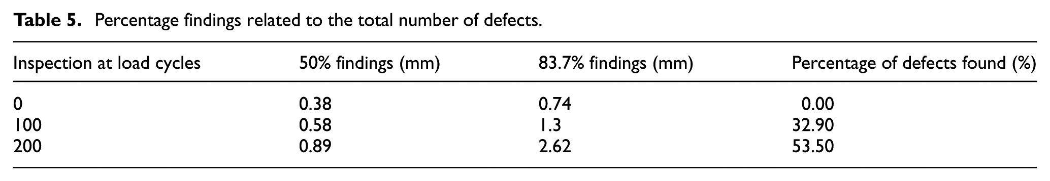
The inspections use the same POD as the original manufacturing inspection lognormal variable PDF a_i. The findings take a shape close to lognormal. The integration of equation (19) (section “Defect size forecasting”) gives the total number of findings equivalent to 32.9% of the defective parts at 100 load cycles. If the process is repeated at 200 load cycles during a second inspection, an additional 20.5% of defective parts are found. The inspections are not fully effective, because of the existence of hidden dormant defects that have not grown yet and the POD of the selected NDT.

A comparison between the number of findings and the size prediction with the real component behavior gives feedback on the readiness level of the inspection method used and the analytical procedure proposed. If the number and size of the findings are lower than those from the analytical prediction, the inspection guarantees target reliability. If not, the inspection plan needs to be changed as proposed in “Repeating loop 1 after loop 4: Update by inspection of probabilistic damage-tolerance assessment.”

Loop 3 part 3: inspection plan

The method in section “Fracture probability and inspection plan” allows for an update of the reliability evaluation based on the inspection and provides a typical saw-tooth reliability graph. The input data are the defect rates that will be found during inspection and the reliability without inspection. As shown in Figure 7, when the failure probability reaches the failure target value, an inspection is necessary to remove defective parts. Then, the procedure is evaluated at two inspection intervals of 100 and 200 load cycles.

Section “Defect rate forecasting” determines an inspection finding rate of 32.9% of the defects in the first inspection at 100 load cycles, then the failure probability decreases below 32.9% because of the removal of defective parts. At 200 load cycles, the rate increases to 53.5%. After removal of the defect, the reliability target is achieved at 300 load cycles. Figure 10 shows the saw-tooth graph, which maintains the failure probability above the target value during component life.

Figure 10.

Failure probability with and without inspection.

Loop 4: inspection findings and welding parameter update

The method in section “Loop 4: probabilistic damage growth model update by inspection findings” uses a likelihood analysis to update the welding parameters. The analysis updates the nominal parameters of Table 2 until the defect size, which is estimated analytically in section “Defect size forecasting” (Figure 9 and “Fleet A” column in Table 6), becomes the 20 inspection findings from the service support process at 100 load cycles. The inspection findings (“Fleet B” column in Table 6) have been calculated by considering the nominal parameters in Table 2 in which component loads σa and σb have been reduced by 20%.

Table 6.

20 defect sizes at 100 load cycles.

Defect number	Probability of defect size exceedance	“Fleet A”		“Fleet B”
Defect number	Probability of defect size exceedance	Defect size (mm)	Failure probability	Defect size (mm)	Failure probability
1	0.048	0.169	0.057	0.141	0.057
2	0.095	0.217	0.084	0.184	0.072
3	0.143	0.259	0.1	0.218	0.084
4	0.19	0.3	0.115	0.251	0.096
5	0.238	0.338	0.129	0.281	0.108
6	0.286	0.377	0.144	0.312	0.119
7	0.333	0.417	0.16	0.342	0.131
8	0.381	0.461	0.178	0.374	0.143
9	0.429	0.503	0.195	0.409	0.157
10	0.476	0.552	0.214	0.445	0.171
11	0.524	0.609	0.238	0.484	0.187
12	0.571	0.672	0.264	0.522	0.202
13	0.619	0.741	0.293	0.572	0.223
14	0.667	0.821	0.327	0.628	0.246
15	0.714	0.91	0.364	0.69	0.272
16	0.762	1.027	0.413	0.765	0.303
17	0.81	1.186	0.478	0.854	0.341
18	0.857	1.406	0.563	0.979	0.393
19	0.905	1.772	0.688	1.16	0.467
20	0.952	2.65	0.875	1.52	0.605

The parameter update is guided and limited by the uncertainty weight of each variable in Table 7, as suggested in section “Loop 4: probabilistic damage growth model update by inspection findings.”

Table 7.

Mean and standard deviation uncertainty parameters.

Relevant parameter group	Relevant parameter	Mean value uncertainty	Standard deviation value uncertainty
Inspections	a_i	1	1
	a_f	–	–
	δ	–	–
Material properties	n	–	–
	c	1	1/20
	K_Ic	–	–
Welding process, geometry, and acceptance criteria	f	1	1/6
	t_w	1	1/33
	e	1	1
	α	1	1
Loads and FEM	σa	1	1
	σb	1	1
	N	–	–
Method uncertainty	λ_w	1	1/10
Method uncertainty	Θ	1	1/10

FEM: finite element model.

During the 100-load cycle inspection, 20 findings were found out of 180 components (which corresponds to a crack occurrence per weld length δ of 5.0 × 10⁻⁵ = 20/π/707/180), and no component failures were reported. As mentioned in section “Loop 4: probabilistic damage growth model update by inspection findings,” the detected crack rate per length unit δ is considered to be tuned and an update is not required.

The outcomes from the method in section “Loop 4: probabilistic damage growth model update by inspection findings” are described below. Table 8 shows the comparison of the sensitivities of the MLE and FWMSV methods applied to “Fleet A” and “Fleet B.” The MLE method evaluates “Fleet A” and “Fleet B” and gives a small sensitivity of 6% ((0.307 – 0.331)/0.399), which is related to the target distance 23% ((0.307 – 0.399)/0.39), because of numerical errors in the FORM + fracture process. The FWMSV evaluation gives a sensitivity of 120% (1.3207 – 0.123), which is 20 times greater than that of the MLE approach, and avoids numerical errors. Thus, FWMSV is used in the remainder of the article for the inspection update.

Table 8.

Adjustment evaluation for different load cases.

	MLE	FWMSV
“Fleet A”	0.307	0.123
“Fleet B”	0.331	1.3207
“Fleet B” update	0.28	0.0007
Target	0.399	0

MLE: maximum-likelihood estimator; FWMSV: failure-weighted mean square value.

The inspection update is based on the “Fleet A” input parameters in Table 2 and the “Fleet B” data. The FWMSV method explained in section “Loop 3: reliability evaluation after inspection” gives the “Fleet B” update evaluation parameters reported in Table 9. The results provide three conclusions: first, the update of the welding parameter standard deviations is negligible compared with the welding parameter mean value contribution; second, the mean value of the material properties c is the most relevant parameter to correct the prediction value; third, several options exist to reach the finding distribution; in this case, the increase in material properties c compensates for the load reduction imposed in “Fleet B.”

Table 9.

Parameters’ mean and standard deviation update proposal.

Relevant parameter group	Relevant parameter	Mean value update need	Standard deviation value update need
Inspections	a_i	0.023	−4.294 × 10⁻³
	a_f	–	–
	δ	–	–
Material properties	n	–	–
	c	0.268	−4.745 × 10⁻⁵
	K_Ic	–	–
Welding process, geometry, and acceptance criteria	f	−0.048	−2.469 × 10⁻⁴
	t_w	0.073	−1.045 × 10⁻³
	e	−0.004	−3.558 × 10⁻⁵
	α	−0.005	−6.253 × 10⁻⁵
Loads and FEM	σa	−0.011	−4.745 × 10⁻⁵
	σb	−0.037	−2.332 × 10⁻⁵
	N	–	–
Method uncertainty	λ_w	0.047	−4.681 × 10⁻⁴
Method uncertainty	Θ	−0.037	−2.513 × 10⁻⁴

FEM: finite element model.

Repeating loop 1 after loop 4: update by inspection of probabilistic damage tolerance assessment

The method in section “Loop 1: reliability evaluation and first inspection schedule” allows for a definition of the inspection based on target reliability. As a first step, the target reliability is established and the welding parameters are defined based on section “Loop 3: reliability evaluation after inspection” (updated by the inspection). Next, the defect growth laws are established as described in section “Crack growth model,” and the reliability evaluation is carried out as explained in section “Fracture limit state function,”“Fatigue limit state function,” and “Fracture probability: FORM + fracture.” Finally, this result is compared with the required reliability and a new inspection schedule is established. In summary, loop 1 is updated after loop 4.

Figure 11 shows an updated welded structure failure probability. The fracture probability curve corresponds to the “Fleet A” parameter evaluation and is the same as that obtained in Loop 1: Probabilistic damage-tolerence assessment. The fracture probability 80% load curve corresponds to the “Fleet B” parameter evaluation that considers a 20% load reduction. The reliability update by inspection curve corresponds to the “Fleet A” parameter update, based on the “Fleet B” findings (parameters in Table 9). As expected, an intermediate line between the “Fleet A” and “Fleet B” curves results.

Figure 11.

Failure probability update.

Repeating loop 3 after loop 4: inspection update

The method in sections “Defect size forecasting” and “Defect rate forecasting” allows for forecasting of the defect size and rate that will exist during inspection. The input data are the welding parameters, defined in section “Loop 3: reliability evaluation after inspection” of this article (updated by the inspection). The procedure is evaluated at 100-load cycle inspection intervals, because the reliability requirement is not fulfilled, as shown in Figure 11 (“reliability update by inspection” graph). The method in section “Fracture probability and inspection plan” allows for an update of the reliability evaluation based on the inspection and provides the typical saw-tooth reliability graph.

Table 10 summarizes the defect rate forecasting and the defect size that overcomes 50% and 83.7% of the defects (mean value and mean plus standard deviation value). The percentage of findings has been evaluated based on section “Defect rate forecasting.” No defects exist at 0 cycles because of the manufacturing inspection, and the percentage of findings increases because of the number of cycles and the load severity. Table 5 in provides an update to consider the “Fleet A” parameter update, based on the “Fleet B” findings (parameters in Table 9). The percentage of findings is reduced from 32.9% to 15.98%, and the reliability is updated by the inspection and the defective part removal as shown in Figure 11. The reliability increase allows for the removal of a second inspection at 200 load cycles (proposed in “Loop 3 part 3: inspection plan”) and the reliability target rate of 1.4 × 10⁻⁴ during 300 load cycles is fulfilled.

Table 10.

Percentage of findings related to the total number of defects.

Welding parameters	Inspection at load cycles	50% findings (mm)	83.7% findings (mm)	Percentage of defects found (%)
–	0	0.38	0.74	0.00
Table 2	100	0.58	1.3	32.90
Table 9	100	0.46	0.92	15.98

Performance of the proposed method

This section compares the performance of the different methods used in the numerical example as explained in this article.

Loop 1: weld reliability forecasting comparison between MCS, FORM, and FORM + fracture

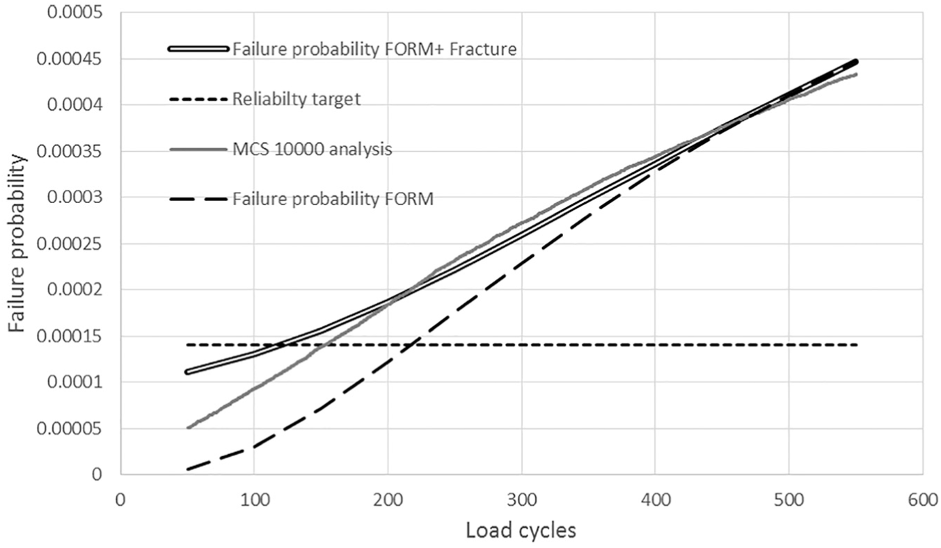
Figure 12 shows the comparison of the results of the conventional FORM (broken line) and the FORM + fracture method (double line) presented in this article. Both methods converge when a typical failure life time is achieved at 530 load cycles. The FORM underestimates the failure probability with a low number of load cycles, because it does not consider the variability of the welding fracture parameters.

Figure 12.

Comparison of FORM versus FORM + fracture versus MCS.

The gray line in Figure 12 adds the 10,000 MCS crack propagation analysis data that is considered the exact solution for the numerical example. The FORM is a nonconservative method because it underestimates the failure probability for all cases. The FORM + fracture method gives a solution closer to the exact solution and is conservative with the necessary reliability requirement.

Loop 2: sensitivity performance

Table 11 shows the comparison of the weld parameters’ reliability sensitivity between the conventional FORM and the FORM + fracture method. The FORM does not consider the variability of the fracture toughness and overpredicts the sensitivity for initial crack size and material properties. For the remaining variables, both methods provide similar values.

Table 11.

Parameter mean sensitivity FORM versus FORM + fracture.

Relevant parameter group	Relevant parameter	Mean value sensitivity FORM + fracture	Mean value sensitivity FORM	Difference (%)
Inspections	a_i	0.473	0.638	−35
	a_f	–	–	–
	δ	–	–	–
Material properties	n	–	–	–
	c	11.041	19.600	−78
	K_Ic	1.510	–	–
Welding process, geometry, and acceptance criteria	f	−4.035	−3.688	9
	t_w	−0.619	−0.634	−2
	e	−0.335	−0.329	2
	α	−0.444	−0.429	3
Loads and FEM	σa	−0.999	−0.912	9
	σb	−3.028	−2.842	6
	N	–	–	–
Method uncertainty	λ_w	3.818	3.677	4
Method uncertainty	Θ	−3.041	−2.852	6

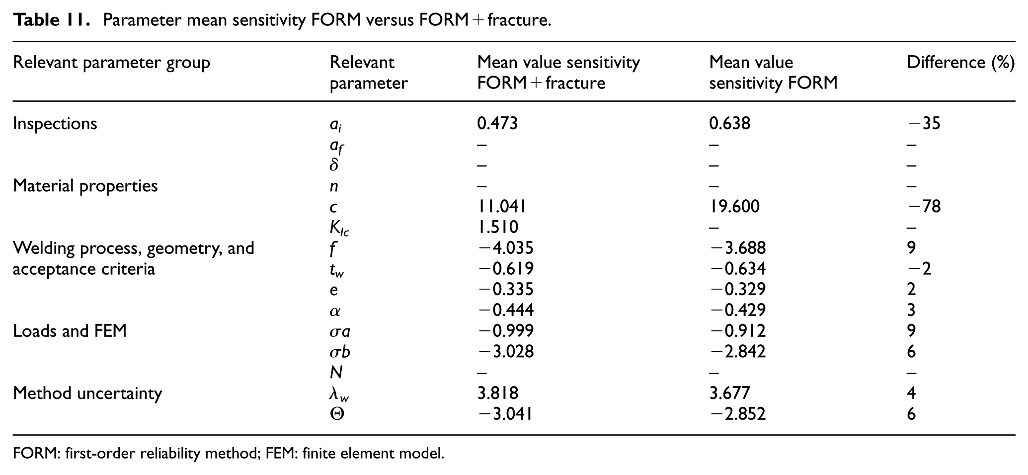
FORM: first-order reliability method; FEM: finite element model.

Loop 3: inspection update

The inspection update is based on reliability evaluation with a constant final crack size, as explained in section “Defect rate forecasting.” As shown in Figure 13, the FORM predicts a good correlation with the 10,000 MCS crack propagation analysis data and is considered the exact solution for the numerical example in parts sections “Loop 3 part 1 and 2: Inspection-finding forecasting” and “Loop3 part 3: Inspection plan”. Figure 14 shows the defect size exceedance probability as a function of the finding size at 100 and 200 load cycles. The graph shows that the FORM predicts a good correlation of the 10,000 MCS crack propagation analysis data (considering the exact solution for the numerical example).

Figure 13.

FORM vs MCS comparison.

Figure 14.

FORM behavior to predict crack size.

Computing efficiency

In the example, the MCS method needs 22,000 crack propagation analyses to achieve a target reliability of 1.4 × 10⁻⁴ with 95% confidence.¹² The FORM + fracture method needs 600 crack propagation analyses, gives an excellent behavior when the failure probability to evaluate is very low, and reduces the computing time 400 times when compared with the reliability evaluation MCS.

Table 12 summarizes the example reported in this article: first, the FORM + fracture needs five crack propagation analyses to evaluate the reliability for a specific number of load cycles (evaluated in 50-load cycle increments from 50 to 550 cycles: 11 × 5 = 55 to construct Figure 7); second, no additional analysis is needed to evaluate the variable sensitivity for all variables; third, a further 11 × 5 = 55 analyses were needed to construct Figure 9 (from a defect size of 0.36 to 10 mm) and to update the inspection plan. Finally, an evaluation of the FWMSV function, which considers 20 defects, needs 5 × 20 = 100 analyses and an update of the input variables based on the defects found needs 5 FWMSV evaluations and 500 crack propagation analyses.

Table 12.

Number of crack propagation analyses.

Method/Simulation type	Reliability	Sensitivity 10 variables	Inspection plan 5 inspections	FWMSV 20 findings
MCS	22,000	0	0	430,000
FORM + fracture	55	0	55	500

FWMSV: failure-weighted mean square value; MCS: Monte-Carlo simulation; FORM: first-order reliability method.

Conclusion

This article presents a novel methodology for the inspection schedule in welded structures. The method is based on a probabilistic crack propagation analysis that updates input parameters to forecast the inspection findings. The uncertainty in material properties, defect inspection capabilities, calculation methods, and loads are considered. The key aspects of the proposed methodology are as follows:

A specific SIF is developed for welds in a plate. The formulation includes the main parameters of weld reliability (inspections, material properties, loads, welding geometry, acceptance criteria, and method uncertainties), which enables the use of elementary functions to solve the Paris law integral.

The conventional FORM was adapted to forecast the defect size with accuracy and to avoid explicit crack growth analyses and MCS.

The proposed novel FORM + fracture method improves the conventional FORM accuracy of reliability calculations significantly and provides results that are similar to the MCS results.

A new finding size likelihood estimator that incorporates structural failure probability was considered, which is more robust than the conventional MLE method.

The associated low computational cost enables the use of the methodology in several areas where probabilistic life calculations have not been implemented yet. During the design of welded structures, an effective design for the manufacturing process can be achieved. Second, the structural health monitoring application that incorporates a defect growth model that learns during the component lifecycle can be developed, which defines a specific inspection for each component. Third, the methodology can be used to develop a damage tolerance crack growth model, which defines improving inspection schedules based on the airplane fleet experience.

Footnotes

Appendix 1 Acknowledgements

We are grateful to the Mechanical Technology Department of ITPAero^® for supporting and helping us with this study. The invaluable guidance and feedback from Jose Ramón Andujar is recognized with great appreciation.

Handling editor: Shun-Peng Zhu

Declaration of conflicting interests

The author(s) declared no potential conflicts of interest with respect to the research, authorship, and/or publication of this article.

Funding

The author(s) received no financial support for the research, authorship, and/or publication of this article.

ORCID iD

Mikel Abasolo

References

Paris

Erdogan

A critical analysis of crack propagation laws. J. Basic Eng 1963; 85: 528–533.

US Department of Transportation. Damage tolerance for high energy turbine engine rotors (AC 33.14-1 Advisory Circular). Washington, DC: Federal Aviation Administration, 2001.

Enright

Millwater

HR.

Probabilistic methods for design assessment of reliability with inspection. AIAA J 2002; 40: 937–946.

Coppe

Pais

Haftka

et al . Using a simple crack growth model in predicting remaining useful life. J Aircraft 2012; 49: 1965–1973.

Kale

Haftka

RT.

Tradeoff of weight and inspection cost in reliability-based structural optimization. J Aircraft 2008; 45: 77–85.

Opgenoord

Willcox

KE.

Sensitivity analysis methods for uncertainty budgeting in system design. AIAA J 2016; 54: 3134–3148.

Millwater

Wieland

DH.

Probabilistic sensitivity-based ranking of damage tolerance analysis elements. J Aircraft 2010; 47: 161–171.

Thoft-Christensen

Murotsu

Application of structural systems reliability theory. Berlin: Springer, 1986.

Madsen

Krenk

Lind

NC.

Methods of structural safety. New York: Dover Publications, 2006.

10.

Feng

Garbatov

Guedes Soares

Fatigue reliability of a stiffened panel subjected to correlated crack growth. Struct Saf 2011; 36–37: 39–46.

11.

Feng

Garbatov

Guedes Soares

Probabilistic model of the growth of correlated cracks in a stiffened panel. Eng Fract Mech 2012; 84: 83–95.

12.

Kapur

Lamberson

LR.

Reliability in engineering design. Hoboken, NJ: Wiley, 1977.

13.

Kim

Pattabhiraman

Houck

. Bayesian approach for fatigue life prediction from field data. In: ASME turbo expo: power for land, sea, and air, Glasgow, 14–18 June 2010, paper no. GT2010-23780, pp.695–703. New York: ASME.

14.

Bhachu

Haftka

Waycaster

et al . Probabilistic manufacturing tolerance optimization of damage-tolerant aircraft structures using measured data. J Aircraft 2015; 52: 1412–1421.

15.

FINET European Fitness-for-Service Network. Selection of failure assessment diagram fracture module. Fracture-fatigue-creep-corrosion. FITNET FFS-GIRT-CT-2001-05071. FINET European Fitness-for-Service (FFS) procedure -Volume 1, 2008, I:6.2.3.2. www.eurofitnet.org

16.

López

Lacalle

Viadero

Hernández

JM.

Applications of dynamic measurements to structural reliability updating. Probabilist Eng Mech 1996; 11: 97–105.

17.

Ditlevsen

Uncertainty modeling. New York: McGraw-Hill Education, 1981.

18.

Viadero

Bueno

López

Lacalle

et al . R: Reliability computation on stiffened bending plates. Adv Eng Softw 1995; 20: 43–48.

19.

MIL-HDBK-1823A. Nondestructive evaluation system reliability.

20.

ASTM E647. Standard test method for measurement of fatigue growth rates.

21.

ASTM E1820. Standard test method measurement of fracture toughness.

22.

Daniewicz

Collins

Houser

DR.

An elastic-plastic analytical model for predicting fatigue crack growth in arbitrary edge-cracked two-dimensional geometries with residual stress. Int J Fatigue 1994; 16: 123–133.

23.

Maddox

. Fitness-for-purpose assessment of misalignment in transverse butt welds subject to fatigue loading. TWI Industrial Member Report, The Welding Institute, Cambridge, July 1985.

24.

Wilson

CD.

Linear elastic fracture mechanics primer. Technical Memorandum 103591, NASA, Washington, DC, July 1992.

25.

Newman

Raju

IS.

An empirical stress-intensity factor equation for the surface cracks. Eng Fract Mech 1981; 15: 185–192.

26.

Sundararajan

Hudak

BY.

Probabilistic structural mechanics handbook: theory and industrial applications. Berlin: Springer, 1995, pp.116–117.

27.

Lee

McClung

Chell

GG.

An efficient stress intensity factor solution scheme for corner cracks at holes under bivariant stressing. Fatigue Fract Eng M 2010; 831: 1004–1016.

28.

Uslu

Demir

Ayhan

AO.

Surface cracks in finite thickness plates under thermal and displacement-controlled loads—part 1: stress intensity factors. Eng Fract Mech 2014; 115: 284–295.

29.

Uslu

Demir

Ayhan

AO.

Surface cracks in finite thickness plates under thermal and displacement-controlled loads—part 2: crack propagation. Eng Fract Mech 2014; 115: 255–269.

30.

FINET European Fitness-for-Service Network. Weld joint stress intensity factor for surface crack at weld toe, 2D FEA based. Fracture-fatigue-creep-corrosion. FITNET FFS-GIRT-CT-2001-05071. FINET European Fitness-for-Service (FFS) Annex -Volume 2, 2008, II:A.6.1.1. www.eurofitnet.org

31.

Melchers

RE.

Structural reliability analysis and prediction. New York; Chichester: Ellis Horwood, 1987.

32.

Smirnov

. A course of higher mathematics: Adiwes international series in mathematics. 1st ed, vol. 1. Oxford: Pergamon Press, 1964, p.512.

33.

Ditlevsen

Bjerager

Methods of structural systems reliability. Struct Saf 1986; 3: 195–229.

34.

Bjerager

On computation methods for structural reliability analysis. Struct Saf 1990; 9: 79–96.

35.

Hasofer

Lind

NC.

Exact and invariant second-moment code format. J Eng Mech 1974; 1: 111–121.

36.

Low

Wilson

Tang

Reliability analysis using object-oriented constrained optimization. Struct Saf 2004; 26: 69–89.

37.

Fox

RL.

Optimization method and engineering design. Method of feasible directions. Boston, MA: Addison-Wesley, 1971, pp.179–195.

38.

Hohenbichler

Rackwitz

Sensitivity and importance measures in structural reliability. Struct Saf 1986; 3: 203–206.

39.

Bjerager

Krenk

Parametric sensitivity in first order reliability analysis. J Eng Mech 1989; 115: 1577–1582.

40.

Enright

Huyse

Methodology for probabilistic life prediction of multiple-anomaly materials. AIAA J 2006; 44: 787–793.

41.

US Department of Transportation. Damage tolerance of hole features in high-energy turbine engine rotor (AC 33.70-2). Washington, DC: Advisory Circular Federal Aviation Administration, 2009.

Inspection scheduling based on reliability updating of gas turbine welded structures

Abstract

Keywords

Introduction

Loop 1: reliability evaluation and first inspection schedule

Inputs: target reliability and welding parameters

Inspections

Material properties

Welding geometry and acceptance criteria

Loads and the finite element method

Method uncertainty

Method: probabilistic damage growth model

Crack growth model

Fracture limit state function

Fatigue limit state function

Fracture probability: FORM + fracture

Loop 2: sensitivity of welding parameters

Loop 3: reliability evaluation after inspection

Defect size forecasting

Defect rate forecasting

Fracture probability and inspection plan

Loop 4: probabilistic damage growth model update by inspection findings

Numerical example: application to gas turbine engine components

Loop 1: probabilistic damage tolerance assessment

Loop 2: weld parameter sensitivity

Loop 3 parts 1 and 2: inspection finding forecasting

Loop 3 part 3: inspection plan

Loop 4: inspection findings and welding parameter update

Repeating loop 1 after loop 4: update by inspection of probabilistic damage tolerance assessment

Repeating loop 3 after loop 4: inspection update

Performance of the proposed method

Loop 1: weld reliability forecasting comparison between MCS, FORM, and FORM + fracture

Loop 2: sensitivity performance

Loop 3: inspection update

Computing efficiency

Conclusion

Footnotes

Appendix 1

Acknowledgements

Declaration of conflicting interests

Funding

ORCID iD

References