Sage Journals: Discover world-class research

Abstract

In this article, we propose a novel scheme for diagnosing intermittent faults for cloud systems. We have investigated the characteristic of high-level symptomatic behavior on top of a cloud system and identified that (1) arrival counts of high-level symptoms go up with the number of fault injections at different speeds, which may help us to differentiate one fault model from another; (2) the nested level of fatal traps is found to be an indicative of fault duration, which is helpful for fault model diagnosis; (3) fatal traps triggered by certain faulty units is explored, providing useful information for locating faults. Based on these features, an n-dimensional space taking symptom’s arrival rate (grown up skew of the arrival count) as each dimension, which formulates the diagnosis problem as a pattern recognition problem is defined. Then, a backpropagation neural-network-based online hardware fault diagnosis scheme is proposed. Experimental results show that diagnosis accuracy of fault location is 99.2%, the accuracy of fault model is 96.7%, and the latency is affordable. This scheme has been implemented in firmware so that it covers cloud software stacks (virtual machine monitor, virtual machines, and user applications) and incurs zero hardware overhead.

Keywords

Cloud computing fault diagnosis neural network

Introduction

The new and emerging generation of cyber-physical systems¹ such as those supported by the Internet of things (IoT)² posed a new set of requirements to computing systems. In these systems, the increasing use of wireless sensors that generate massive data and the need to process these data efficiently have given an enormous importance to the cloud computing paradigm. A good example of cyber-physical applications are those running in the context of vehicular ad hoc networks (VANETs).³ In these systems, drivers are offered a set of services which might involve congestion information, parking place management, entertainment, vehicle tracking, and so on. Applications of this type need not only to run efficiently (therefore expecting fast processing and storage) but also to be reliable. These cyber-physical systems require real-time processing, efficient storage, and accessibility and other non-functional requirements such as reliability. Reliability refers to the probability of a system, including all of its hardware and software components, to perform correctly as expected.

At the same time, new trends in semiconductor technology scaling toward a nanometer regime have impelled a resurgence of interest in detecting and diagnosing intermittent faults. The driving forces⁴ include shrinking geometries, smaller interconnect dimensions, lower power voltages, decreased noise margins, and so on. It has been forecasted that multicore and manycore systems, mostly often integrated in cloud systems build schemes, are more vulnerable to intermittent faults in future technologies.⁵

Unlike transient faults due to single-event upset (SEU), intermittent faults occur in bursts with durations that vary across a wide range of timescales, from orders of cycles, to milliseconds, to even seconds or more. As compared with permanent faults, intermittent faults do not persist and are hard to diagnose through periodic tests because they arise in particular situations (temperature, supply voltage, voltage droops, and so on) and cannot be reproduced.⁶

Error-correcting codes (ECC) or parity is generally used to protect sequential logic from intermittent fault, but they are not suitable for diagnosis or fault detection of combinational logic. Prior works such as triple modular redundancy (TMR) or hot spare systems have been shown to be effective, but are considered unaffordable in many scenarios. Online testing and SBST (software-based self-test) are promising not only for sequential logic from erratic bits⁷ but also for combinational logic.^8–10 However, the burst and non-recurrence features make SBST no longer effective for intermittent faults.¹¹

Li et al.¹² developed a set of high-level fault detection mechanisms. High-level detection techniques generally ignore faults which are masked at any of these levels, avoiding the corresponding overheads. Compared to the low-level mechanisms, it achieves low cost, low misdiagnosis rate, but longer delays. However, the effectiveness for covering intermittent faults has not been verified. And, the diagnosis version (m-SWAT)¹³ incurs high overhead, and it is only suitable for permanent faults.

In this article, we propose a fault diagnosis strategy for combinational logic in processors against intermittent faults. The diagnosis strategy fundamentally depends on the answers to several key questions, which we investigate in this work:

Are detection mechanisms effective for combinational logic under intermittent faults? First, the mechanisms should cover all three fault models (transient, intermittent, and permanent). In addition, the detection delay must be reasonable to provide timing margin for diagnosis and recovery mechanisms.

Different fault models last for different time lengths, which may result in various symptoms of cloud systems. What is the relationship between fault models and symptoms we can detect? This may provide useful information for fault diagnosis.

Is there an inherent connection between symptoms and fault components? If so, understanding the connection may be helpful to determine the fault location.

To answer these questions, we have investigated high-level symptomatic behaviors by exploiting traces in fault injection campaigns, based on a cloud system simulating environment. Then, we observed three features of symptom behavior which are vital for the fault diagnosis process. Finally, an online hardware fault diagnosis system based on neural network has been devised, and it is proposed in this article. Our contributions are as follows.

Three features of symptomatic behavior have been observed from further analysis. (1) Arrival counts of fatal traps and high activities go up with the number of fault injections at different speeds, which allows defining an n-dimensional space using the arrival rate of each symptom as coordinates in which the training samples will gather into clusters. As a result, the diagnosis strategy can be treated as a pattern classification problem so that a neural network is employed. (2) Nested level of fatal traps is directly related to fault duration, which helps to distinguish fault models. (3) Dedicated fatal traps contribute to structure-level fault location.

A Backpropagation (BP)-based OnlIne hardware fault Diagnosis System has been built, named BOIDS, which is used to diagnose combinational logics in microprocessors against hardware faults (transient, intermittent, and permanent faults) in cloud computing environments. The diagnosis scheme is implemented in the firmware layer so that it can be easier to modify, thus saving cost to trade-off performance with reliability without requiring any change to the underlying hardware. It also allows the neural network algorithm to diagnose online, while the exhausting training process can be dealt offline, therefore saving significant upgrading overhead. Experimental results show that diagnosis accuracy of fault location is 99.2% and accuracy of fault model diagnosis is 96.7%, with latency favorable for hardware recovery mechanisms.

To our knowledge, this article makes the first attempt toward diagnosing hardware faults in cloud systems using neural networks. This scheme shows acceptable diagnosis accuracy and low hardware overhead which benefits from features of symptomatic behavior observed in the statistical analysis of the injection experiment. This scheme diagnoses not only fault models (transient, intermittent, and permanent) but also the fault locations in combinational logics, such as address generation unit (AGEN), decoder, arithmetic logic unit (ALU), and float point unit (FPU).

This article is organized as follows: section “Related work” describes related work; section “Features of symptomatic behavior” presents features of high-level symptomatic behaviors; section “Design of BOIDS” presents the design of BOIDS; section “Experimental results” shows the evaluation of the diagnosis scheme; and section “Conclusion” concludes the article.

Related work

In this section, we present prior research in hardware fault diagnosis. In recent years, much work has been done on studying the impact of intermittent faults on computer systems.^14,15 L Rashid et al.¹⁶ made a preliminary study of intermittent fault propagation in programs, and J Wei et al.¹⁷ further his study. Gracia-Moran and colleagues^18,19 evaluated redundancy-based fault tolerance capabilities for intermittent faults. Pan et al.²⁰ introduced intermittent faults vulnerability factor (IVF) to quantitatively investigate vulnerability of processor structures against intermittent faults.

Traditional fault resilient techniques are usually based on adding redundancy or using voters, such as in the IBM mainframes.²¹ The IBM G5 microprocessor, for example, has redundant units for fetch/decode and for instruction execution. Some other fault-tolerant computers, such as the Stratus²² and the Tandem S2,²³ simply replicate entire processors. An even more extreme case of using redundancy to tolerate fabrication defects is the Teramac.²⁴ The Teramac is designed to make use of components that are likely to be faulty and has been motivated by expected defect rates in nanotechnology. While all these systems provide excellent resilience to hardware faults, such heavyweight redundancy incurs significant costs in terms of hardware and power consumption.

Several techniques provide firmware access to the processor’s internal state in order to detect hardware faults by periodical tests.²⁵ However, such methods may not be effective due to the non-periodical characteristic of intermittent faults.

Symptom-based fault detection has been proposed by ML Li et al.¹² This is an effective detection technique for permanent and transient faults in an operating system scenario. Compared to our method, the effectiveness of this method remains untested neither for intermittent faults nor for the cloud computing environment. We believe that after validation of its effectiveness, the method can be introduced into our scheme as a pre-step for fault diagnosis process, and the log trace can also be used by our fault diagnosis scheme.

Several methods to continue use of a core despite permanent faults have been published. These techniques involve fine-grained diagnosis and reconfiguration of a core’s components,^26,27 or attempt to match program requirements and with core capabilities, such as Core Salvage.²⁸ PM Wells et al.²⁹ believed that the ability to suspend execution on a core, in order to perform diagnosis and reconfiguration, would likely be a simplifying addition to these techniques.

S Hari et al. designed a trace-based fault diagnosis (TBFD) mechanism to diagnose permanent faults. Although the diagnosis accuracy reaches 95%, heavyweight overheads such as hardware buffers and re-executions are required.³⁰ Furthermore, TBFD does not show its effectiveness for intermittent faults, taking into account of the burst and non-periodical characteristics of intermittent faults.

Features of symptomatic behavior

Neural networks are widely known for their performance in the pattern recognition area due to their ability to partition a non linear sample space. We have investigated high-level symptomatic behaviors and extracted three features to employ as a fault diagnosis scheme.

Introduction of high-level symptoms

A fatal trap is a special kind of trap thrown by the trap logic unit (TLU) indicating a system in emergency. A fatal trap requires no additional hardware overhead. On Solaris, the following traps are denoted as fatal traps: Recover Error and Debug (RED) state trap (thrown when there are too many nested traps), Data Access Exception trap, Division by zero trap, Illegal instruction trap, Memory misaligned trap, and Watchdog reset trap (thrown when no instruction retires in the last 216 ticks).

High activity refers to the amount of time the execution remains in the operating system without returning to the application. This mechanism has been developed by Li et al.¹² and incurs low hardware overhead, since it primarily uses a hardware instruction counter. The threshold has been set to be 7000 instructions for hypervisor and 30,000 for operating system, which are 1.5 times the normal situation. Note that the number of contiguous instructions does not include system calls or operating system idle state.

Hang is an endless loop or waiting for an event that will never happen. Note that hang is not employed in our diagnosis system since few hangs (0.1%) take place in the detection process. The uncovered proportion is taken by silent data corruption (SDC) that represents faults that manage to survive all the detection barriers and finally result in incorrect results. We can see that longer fault durations induce greater destructive power in the high-level (e.g. in the operating system) and cause more faults to manifest such that they are detected as high-level symptoms.

Statistical methods of high-level symptoms

In what follows, we show that the arrival counts of high-level symptoms, including all the fatal traps and high activities, go up with the number of fault injections, approximately linearly with various slopes. If we setup an n-dimensional space taking the symptom’s arrival rate (grown up skew of the arrival count) as each dimension, the vectors—representing symptoms induced by different fault models and locations—may gather into clusters in the sample space, and the symptom-based diagnosis problem can be treated as a pattern classification problem.

In order to relate symptoms to training patterns, we define the notion of arrival count to represent the number of times that one symptom takes place in the fault injection history. Figure 1 shows the arrival counts of high-level symptoms. First, we made statistics on the fatal traps in fault injections. As we have two diagnosis targets here, the fault model and fault location, we lock one target and observe the change of data under another one in order to “show” the differences of the raw data. In Figure 1, the arrival counts of fatal traps are shown in a two-dimensional (2D) space and each of them are accumulated from 300 faulty traces.

Figure 1.

Arrival counts of symptoms: (a) benchmark: basicmath, structure: decoder, transient/intermittent/permanent; (b) location diagnosis, under intermittent faults and across benchmarks.

The arrival counts of illegal_instruction (fatal trap type: 0x10) and mem_address_not_aligned (fatal trap type: 0x34) from basicmath under a faulty decoder are shown in Figure 1(a). There are three sets of data in a combination of 0x10 and 0x30 and six curves in total, which shows statistics under transient, intermittent, and permanent failures, respectively. We can see that the arrival counts go up with the number of fault injections, and the slopes of the curves are different (strictly speaking, these are not straight lines statistically). It shows us that the growing pace of fatal traps can differentiate one fault model from another, even by the same fatal trap. The T:10, representing the arrival count of fatal trap 0x10 from a transient fault, goes up slower than the I:10, and the arrival count of 0x10 from an intermittent fault (I:10) is slower than that of P:10 (0x10 from a permanent fault). We can also find the difference in fatal trap 0x34 for the three fault models. As a consequence, we can differentiate fault models using grown-up trends of arrival counts of fatal traps occurring in cloud systems in case of faults.

Figure 1(b) also shows arrival counts of fatal traps in each 300 faulty traces, which come from under intermittent faults and all three faulty structures, respectively. However, curves in this figure are the statistics (in average) of trace data generated by all the benchmarks. It can be seen that the curves in Figure 1(b) have higher linearity than those in Figure 1(a), indicating that the characteristics of arrival counts grown trend are more consistent in various user programs. Note that the arrival counts are distinguishable across fault locations, including AGEN, decoder, ALU, and FPU. The fatal trap 0x34 under a faulty decoder (Decoder:34) arrives faster than that of ALU:34, while the arrival count of fatal trap 0x10 from decoder and AGEN are relatively close. However, we can enhance the discrimination by exploiting other fatal traps, such as Decoder:34 and AGEN:10. For decoder, fatal trap 0x34 occurs more than 60 times in each 300 fault injection group, while for AGEN, there are almost none (hence not shown in Figure 1(b)); a similar situation occurred for fatal trap 0x10 for AGEN and decoder. Usually, there are tens of fatal traps in cloud systems and so we can further distinguish the fault locations by making use of more symptoms. As a result, this feature draws a more general feature of fatal traps in order to help fault location diagnosis, particularly in complex computing environments like cloud systems.

Then, if we define an n-dimensional space using the arrival rate (the grown-up skew of the arrival count) of each fatal trap as coordinates, the training samples gather into clusters. Figure 2 shows a 2D space using the arrival rates of 0x10 and 0x34 as coordinates. We can see that the fatal trap sequence, triggered in each type of failure, gathers in clusters in the sample space, and the sample space of symptomatic behavior in the cloud system can be divided if we use the arrival rate of each fatal trap as training pattern. Over all, the proposed statistical method shows the feasibility in setting up a classifier for the sample space of the high-level symptom’s arrival rates, which is the foundation for our diagnosis method.

Figure 2.

The samples of symptoms (0x10 and 0x34) in 2D space: “0” for transient, “x” for intermittent, and “.” for permanent faults.

Nested fatal traps

Intermittent faults are caused by a variety of factors and typically last for a range of durations. In this section, we present a quantitative analysis to understand the relationship between fault models and fault durations.

From fault traces, we found another symptomatic behavior—nested fatal traps. In normal execution flows, fatal traps will not take place, not to mention nested fatal traps. However, when a fault is provoked, especially with longer durations, fatal traps may be triggered before the prior fatal trap returns. We call such cases nested fatal traps. Fault traces show that nested fatal traps take a proportion of 53% in all fatal trap symptoms.

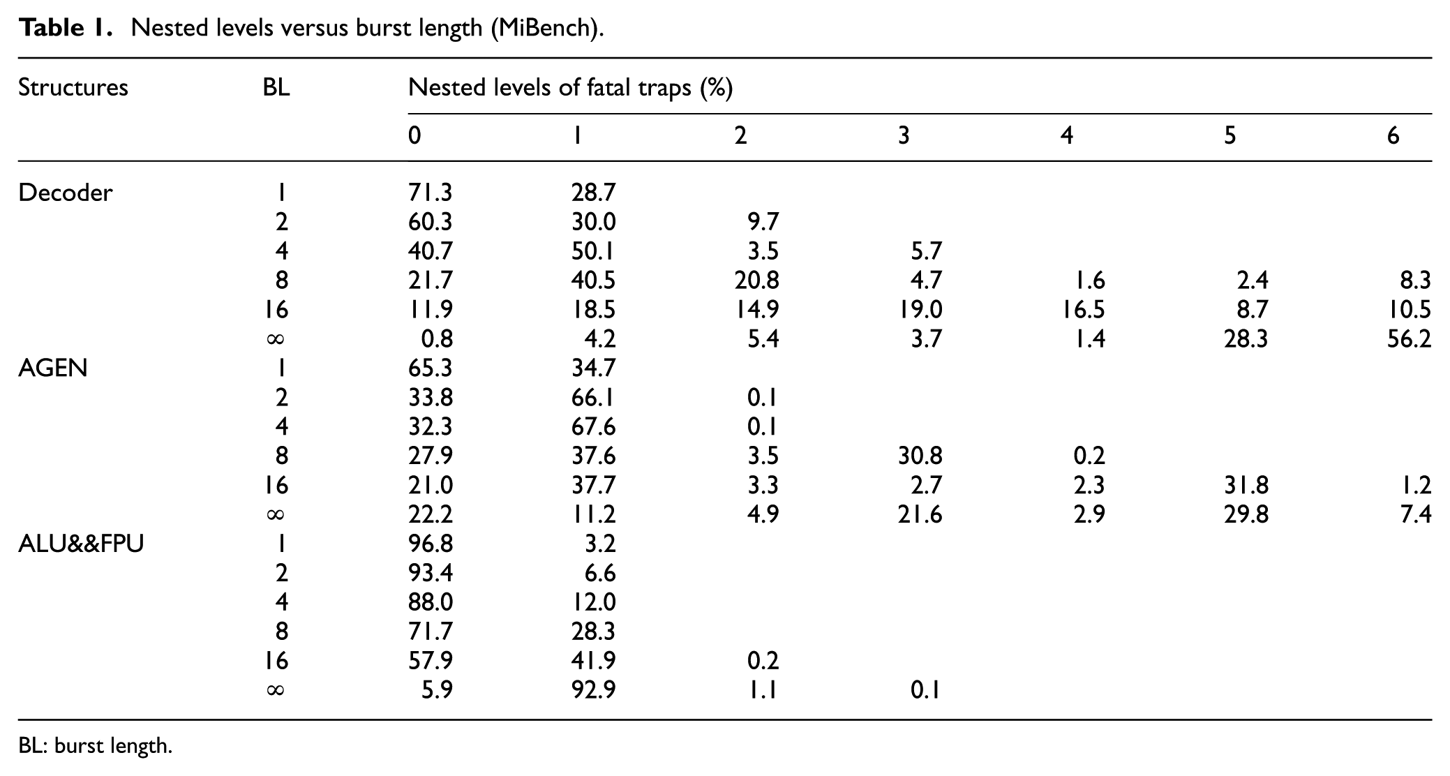
Table 1 shows nested levels of fatal traps versus burst length (BL) for the MiBench benchmark.³¹ There are seven nested levels because the maximum nested level is set to 6 in the UltraSparc system. Level “0” indicates that no fatal traps have occurred, so the figures represent the proportions of high activity. The BL column represents fault durations in fault models, in which “1” corresponds to transient faults, “∞” corresponds to permanent faults, and “2” ∼ “16” correspond to intermittent faults. We can see that the increase in the nested level is directly related to BL. All fatal traps are non-nested in case of a transient fault, while the max nested levels rise from 2 to 6 when intermittent faults occur. Even for the ALU, in which fatal trap detectors show the worst performance, the nested level goes up to 3 when permanent faults occur.

Table 1.

Nested levels versus burst length (MiBench).

Structures	BL	Nested levels of fatal traps (%)
Structures	BL	0	1	2	3	4	5	6
Decoder	1	71.3	28.7
	2	60.3	30.0	9.7
	4	40.7	50.1	3.5	5.7
	8	21.7	40.5	20.8	4.7	1.6	2.4	8.3
	16	11.9	18.5	14.9	19.0	16.5	8.7	10.5
	∞	0.8	4.2	5.4	3.7	1.4	28.3	56.2
AGEN	1	65.3	34.7
	2	33.8	66.1	0.1
	4	32.3	67.6	0.1
	8	27.9	37.6	3.5	30.8	0.2
	16	21.0	37.7	3.3	2.7	2.3	31.8	1.2
	∞	22.2	11.2	4.9	21.6	2.9	29.8	7.4
ALU&&FPU	1	96.8	3.2
	2	93.4	6.6
	4	88.0	12.0
	8	71.7	28.3
	16	57.9	41.9	0.2
	∞	5.9	92.9	1.1	0.1

BL: burst length.

Furthermore, with the increment of fault duration, the proportion of low nested level symptoms (lower than 3) decreases sharply, whereas a reverse trend is observed for higher levels, from 3 to 6. Take decoder as an example: 40.53% of symptoms are non-nested fatal traps when the BL is 8, and the figure decreases to 18.47% when the BL goes to 16. For permanent faults, the proportion goes deep down to 4.20%. But in level 5, the proportion goes up from 2.27% to 28.27% corresponding to an increment of BL.

The above discussion shows how the maximum level and proportion in each level help to distinguish fault models. Furthermore, the speedup ratios of proportion decrement for each structure also show their contribution for fault location. The proportions of symptoms, including high activity, decrease when fault duration increases. Figures from nested level “0” show that the proportion of high activity for decoder goes down linearly. However, the curves of speedup ratio for AGEN, ALU, and FPU change in different ways.

Dedicated fatal trap

The third characteristic of symptomatic behavior is that there are some dedicated fatal traps. We define dedicated fatal traps as those fatal traps that are triggered only by a certain faulty structure (never by others), and this behavior remains inconsistent with all fault models. Obviously, this observation is helpful for fault location.

Dedicated fatal traps are shown in Table 2. In column 3, all the fatal traps dedicated to a corresponding structure are listed (five for decoder, two for AGEN, and none for ALU). For the ALU, each dedicated trap has been triggered a number of times. To show the frequency, the triggering for all fatal traps is listed in the “fatal trap” column. Although some of the frequencies are low, under the assumption that only one fault is provoked at a time, the faulty structure can be located immediately when a dedicated fatal trap occurs.

Table 2.

Dedicated fatal traps for SpecInt2000 (in bold) and MiBench.

Fault model	Structure	Dedicated fatal traps					Fatal traps
Intermittent	Decoder	0x37(39)	0x38(1)	0x20(1)	0x35(1)	0x36(1)	3733
Intermittent	AGEN	0xa(81)	0xd(1290)				2488
Permanent	Decoder	0x37(9)	0x38(0)	0x20(18)	0x35(1)	0x36(2)	1407
Permanent	AGEN	0xa(18)	0xd(382)				1194
Transient	Decoder	0x37(6)	0x38(0)	0x20(0)	0x35(0)	0x36(0)	732
Transient	AGEN	0xa(0)	0x0d(313)				904

Note: Bold values are statistics from testbench SpecInt2000, and unbold values in “Dedicated fatal traps” are statistics from testbench MiBench.

Note that some traps have not taken place in all fault models, but they still meet the definition of dedicated fatal trap. This is the reason why fatal traps that are triggered for zero times are still listed here. The emergence of dedicated fatal traps reveals some internal relationships between the error protection strategy and symptoms (fault manifestations). By making use of dedicated fatal trap, we will solve the diagnosis problem.

Design of BOIDS

Based on the observations of symptomatic behavior, a BP-based online intermittent fault diagnosis system, named BOIDS, for cloud computing systems has been implemented. In this section, we describe the design and implementation of the BOIDS system.

BOIDS comprises four main sub-systems: Symptom Collection Unit (SCU), BP neural network (BPNN from now on), the Arbitrator, and the Fault Recovery Unit (FRU), as depicted in Figure 3. The SCU is responsible for collecting symptoms reported by high-level symptom detectors in case of hardware faults. The SCU maintains the number of times for each symptom and then constitutes the input vector for the BPNN. In case of a fatal trap, the SCU also needs to obtain the nested level from the Trap Level Register (a status register in processor) and look up the dedicated fatal trap table to identify whether it is a dedicated fatal trap or not. The BPNN acquires symptoms from the SCU, makes the recognition, and delivers results to the Arbitrator. In each diagnostic cycle, the BPNN takes an 8-dimensional vector X as input. Each x_i, i = 0 to 7, is one of the seven arrival rates (six fatal traps and high activity) or nested level of symptoms. Since there are three fault models and three candidate structures, nine fault classifications are employed. The BPNN outputs an 8-dimensional vector corresponding to nine fault classifications. In the output vector, a negative value is interpreted as a classification hit. A non-negative value is interpreted as a classification miss. The Arbitrator takes the recognition results of the BPNN as inputs and identifies the pattern of results first. If there are no positives (undiagnosed faults) or more than one positive (non-uniquely identified fault) in the pattern, the result is incorrect. In these cases, the dedicated fatal trap is used to correct the results. Otherwise, incorrect results could still exist, even if the signal pattern is correct. These cases are named uniquely diagnosed faulty results and cannot be identified simply by result patterns. In such situations, continuous symptoms will take place and be detected, and then the Arbitrator suggests adjusting the weights of the BPNN and indicates a new diagnosis cycle.

Figure 3.

The design of BOIDS.

The cross-layer resilient framework provides a large design space by exploiting a series of state-of-the-art techniques across different system stack layers for fault validation and recovery. Mechanisms such as checkpointing,^32,33 migration,³⁴ and reconfiguration³⁵ would be effective and provide enhancement in intermittent fault validation. Further analysis of these issues is out of the scope of this article, so the evaluation of BOIDS is based on the assumption that the cross-layered validation is ideal.

Experimental results

In this section, we show the diagnosis performance of BOIDS against hardware faults for cloud computing systems. We evaluate BOIDS by doing fault injection experiments on a cloud computing simulation environment, in which hardware faults in the processor can be emulated and the reaction of the diagnoser can be monitored.

Experiment methodology

The primary objective of this study is to investigate the features of high-level symptoms, if any, in order to solve the diagnosis problem. This requires simulators which can faithfully simulate system-level software stacks. While alternative field-programmable gate array (FPGA)-based emulations^36–38 offer higher speed and model lower-level faults with high fidelity, their limited observability and controllability gives less flexibility than software simulations.¹² While simulated fault injections^39,40 can accurately capture lower-level faults, the long simulation time of these schemes prevents detailed evaluation of the propagation of faults through the hardware and into the software. We developed a fault injection platform incorporating a full system simulator, SAM,⁴¹ which simulates Ultrasparc T2. On top of SAM lays the cloud system software stack including hypervisor, GuestOS, and user applications. This simulation setup allows us to inject hardware faults into the ALU, AGEN, and decoder and to observe their impact on real workloads (8 SpecInt2000 and 10 MiBench) running on the cloud system.

We have adopted the most commonly used models, such as stuck-at (0, 1) for permanent faults and bit flip for transient faults. Intermittent faults are similar to transient faults, except for their burst characteristics. Once an intermittent fault is activated, every instruction passing the target structure is corrupted until burst ceases. We adopted bit flip fault models with BL s as 2/4/8/16 continuous instructions for intermittent faults.^16,42 Fault injection locations of each target structure are listed in Table 3. In all cases, we have injected single bit faults.

Table 3.

Target units and corresponding fault locations.

Units	Fault locations
Decoder	Instruction decode buffers
ALU_FPU	Input Latch of ALU and FPU
AGEN	Output Latch of Address generation unit
Register file	Bits in register file

Decoder: decoder unit, which is responsible for decoding instructions and generating control signals. ALU_FPU: Integer arithmetic logic and floating point unit. Note that both of integer and floating point instructions’ format are parsed in FBT and thus the evaluation covers the operations in ALU and FPU. AGEN: Address generation unit, a key unit for instruction sequence used to generate the memory address of the next executed instruction.

Representative benchmarks from SpecInt2000 and MiBench have been selected. For each configuration, 300 fault injections have been conducted. Overall, a total of 64,800 runs (300 injections × 3 structures × 18 benchmarks × 4L_burst) for intermittent, 32,400 runs for permanent, and 16,200 runs for transient faults have been conducted. The processor simulator was set in 1c1t (1 core 1 thread) configuration. Since multicore diagnosis is more complex, corresponding configurations are left for our future work.

Diagnosis accuracy

We conducted over 1,000,000 diagnosis experiments and assume that there is only one faulty structure under a specific fault model in each of them. Since this article focuses on intermittent fault diagnosis mechanisms on behalf of fatal trap symptoms, the following evaluation is under the assumption that the performance of the underlying fault validation technology is ideal.

Experimental results show excellent diagnosis accuracy of our diagnosis system. Table 4 shows the accuracies of the first diagnosis cycle since there may be more diagnostic cycles in case of misdiagnosis. In fact, the diagnosis accuracy will definitely go up when the number of diagnosis cycle increases. The statistics of five benchmarks from MiBench are listed, while others are not shown due to the scope limitation.

Table 4.

Diagnosis accuracy for first time diagnosis (MiBench).

Bench	Permanent fault						Intermittent fault						Transient fault
	ALU&&FPU		Decoder		Agen		ALU&&FPU		Decoder		Agen		ALU&&FPU		Decoder		Agen
	struc	model	struc	model	struc	model	struc	model	struc	model	Struc	model	struc	model	struc	model	struc	model
Basi	99.7	99.0	99.3	99.3	99.3	99.3	99.0	74.2	98.8	94.6	99.5	99.5	90.0	80.0	100.0	99.2	99.6	100.0
Dijk	100.0	99.7	100.0	85.9	99.7	100.0	98.6	98.7	99.8	97.9	99.5	99.5	98.2	0.0	95.5	100.0	100	99.6
FFT	100.0	100.0	99.0	93.4	99.3	99.0	99.6	97.8	99.1	99.1	99.1	99.6	96.2	46.2	98.5	96.9	97.7	99.2
Qsor	100.0	100.0	100.0	99.3	100.0	99.0	99.6	98.5	99.1	95.4	95.4	98.7	100.0	87.9	98.7	99.4	94.2	100.0
Strin	99.0	99.3	100.0	95.8	99.3	99.0	98.6	96.6	99.3	92.1	92.1	99.5	100.0	70.8	100.0	84.8	99.2	99.6

From Table 4, we can see that most of diagnosis accuracies are excellent, for both fault model diagnosis (“model” column) and structure-level fault location (“struc” column). The average accuracy of fault location is 99.2% and the accuracy of model diagnosis is 96.7%.

However, the accuracy of transient faults (97.9% for locating and 84.2% for fault model) declines sharply in comparison with that of intermittent fault (99.3% and 98.1%) and permanent faults (99.6% and 97.9%). The similarity of intermittent faults with BL 2 and transient faults may be a rough reason. However, transient faults will disappear during a second-time diagnosis in case of first time misdiagnosis. Accordingly, the disappearance of symptoms will help to increase accuracy.

Diagnosis latency

Diagnosis latency is a crucial parameter since it determines the recovery strategy. According to the architecture of our diagnosis system, a diagnosis result is generated within 1 K instructions after fault detection. Accordingly, a hardware recovery mechanism is feasible.

Conclusion

In this article, we proposed an intermittent fault diagnosis system that employs neural network methods—BP in particular—as a diagnosis scheme. By investigating the characteristics of high-level symptoms, we have found that the statistical method shows the possibility of setting up a classifier for the sample space of high-level symptom’s arrival rates. This formulates the hardware fault diagnosis problem as a pattern recognition problem.

In addition, we observe that (1) the nested level of fatal traps can be used as an indicator for fault duration, which is helpful for fault model diagnosis, and (2) fatal traps triggered by certain faulty structures, named dedicated fatal trap, are useful for fault location. These two observations provide methods to improve the fault diagnosis scheme.

Experimental results show that diagnosis accuracy of fault location is 99.2% and accuracy of fault model diagnosis is 96.7%, while fault detection coverage reaches over 97.2% for SpecInt2000 and 95.1% for the MiBench benchmark. The latency of BOIDS provides opportunities for lightweight recovery techniques.

To the best of our knowledge, we have made a first attempt on intermittent fault diagnosis scheme of cloud systems using the arrival rate of high-level symptomatic behavior to setup the sample space. In a future work, we propose to expand the scheme to more complex scenarios, such as multithread computing environments and virtual machine migration processes. Finally, we would also like to couple this diagnosis framework with recovery techniques both online and offline.

Footnotes

Handling Editor: Fei Yu

Declaration of conflicting interests

The author(s) declared no potential conflicts of interest with respect to the research, authorship, and/or publication of this article.

Funding

The author(s) disclosed receipt of the following financial support for the research, authorship, and/or publication of this article: This work was financially supported by the Natural Science Foundation of Beijing (4174091), Research Funds for Education Committee of Beijing (KM201711232013), and Key Research Project of Beijing Natural Science Foundation (Z16002).

ORCID iD

Chao Wang

References

Wolf

Cyber-physical systems. Computer 2009; 42: 88–89.

Chaari

Ellouze

Koubâa

et al . Cyber-physical systems clouds: a survey. Comp Networks 2016; 108: 260–278.

Wang

Vehicular ad hoc networks. In: Misra

Zhang

Misra

(eds) Guide to wireless ad hoc networks: Computer communications and networks. London: Springer, 2009, pp. 503–525.

Ghobadi

Karimi

Heidari

et al . Modeling the effect of technology trends on soft error rate of combinational logic. In: Proceedings international conference on dependable systems and networks (DSN), Bethesda, MD, 23–26 June 2002. New York: IEEE.

Wells

Chakraborty

Sohi

GS.

Adapting to intermittent faults in multicore systems. In: Proceedings of international conference on architectural support for programming languages and operating systems (ASPLOS), Seattle, WA, 1–5 March 2008. New York: IEEE.

Smolens

Gold

Hoe

et al . Detecting emerging wearout faults. In: IEEE workshop on silicon errors in logic system effects, Austin, TX, 3–4 April 2007. New York: IEEE.

Vera

Abella

Carretero

et al . Online error detection and correction of erratic bits in register files. In: 15th IEEE international on-line testing symposium (IOLTS), Lisbon, 24–26 June 2009. New York: IEEE.

Abella

Vera

Unsal

et al . Fuse: a technique to anticipate failures due to degradation in ALUs. In: 13th IEEE international on-line testing symposium, Crete, 8–11 July 2007. New York: IEEE.

Carretero

Vera

Abella

. A low-overhead technique to protect the issue control logic against soft errors. In: 5th workshop on silicon errors in logic—system effects (SELSE), Stanford University, Stanford, CA, 24–25 March 2009. New York: IEEE.

10.

Carretero

Vera

Chaparro

et al . On-line failure detection in memory order buffers. In: IEEE international test conference (ITC), Santa Clara, CA, 26–31 October 2008. New York: IEEE.

11.

Abella

Chaparro

Vera

et al . On-line failure detection and confinement in caches. In: Proceedings of IOLTS, Rhodes, 7–9 July 2008. New York: IEEE.

12.

Ramachandran

Sahoo

et al . Understanding the propagation of hard errors to software and implications for resilient system design. In: Proceedings of international conference on architectural support for programming languages and operating systems (ASPLOS), Seattle, WA, 1–5 March 2008. New York: IEEE.

13.

Ramachandran

Sahoo

et al . Trace-based microarchitecture-level diagnosis of permanent hardware faults. In: Proceedings of the 38th international conference on dependable systems and networks (DSN), Anchorage, AK, 24–27 June 2008. New York: IEEE.

14.

Constantinescu

. Intermittent faults and effects on reliability of integrated circuits. In: Proceedings of international symposium on reliability and maintainability (RAMS), Las Vegas, NV, 28–31 June 2008. New York: IEEE.

15.

Gil-Tomas

Saiz-Adalid

Gracia-Moran

et al . Injecting intermittent faults for the dependability validation of commercial microcontrollers. In: HLDVT’08, Incline Village, NV, 19–21 November 2008, pp.177–184. New York: IEEE.

16.

Rashid

Pattabiraman

Gopalakrishnan

. Towards understanding the effects of intermittent hardware faults on programs. In: International conference on dependable systems and networks workshops (DSN-W), Chicago, IL, 28 June–1 July 2010. New York: IEEE.

17.

Wei

Rashid

Pattabiraman

et al . Comparing the effects of intermittent and transient hardware faults on programs. In: International conference on dependable systems and networks (DSN), Hong Kong, China, 27–30 June 2011. New York: IEEE.

18.

Gracia-Moran

Saiz

Baraza

et al . Analysis of the influence of intermittent faults in a microcontroller. In: Proceedings of workshop on design and diagnostics of electronic circuits and systems, Bratislava, 16–18 April 2008. New York: IEEE.

19.

Gracia-Moran

Gil-Tomas

Saiz-Adalid

et al . Experimental validation of a fault tolerant microcomputer system against intermittent faults. In: Proceedings of IEEE/IFIP international conference on dependable systems and networks (DSN), Chicago, IL, 28 June–1 July 2010. New York: IEEE.

20.

Pan

. IVF: characterizing the vulnerability of microprocessor structures to intermittent faults. In: Proceedings of IEEE/ACM conference on design, automation and test in Europe, Dresden, 8–12 March 2010. New York: IEEE.

21.

Spainhower

Gregg

TA.

IBM S/390 parallel enterprise server G5 fault tolerance: a historical perspective. IBM J Res Dev 1999; 43: 863–873.

22.

Wilson

The Stratus computer system. In: Schagaev

Castano

(eds) Resilient computer systems. London: Springer, 1985, pp.208–231.

23.

Jewett

Integrity S2: a fault-tolerant UNIX platform. In: Proceedings of the 21st international symposium on fault-tolerant computing systems, Montreal, QC, Canada, 25–27 June 1991, pp.512–519. New York: IEEE.

24.

Culbertson

Amerson

Careter

et al . The Teramac custom computer: extending the limits with defect tolerance. In: Proceedings of the IEEE international symposium on defect and fault tolerance in VLSI systems, Washington DC, USA, 6–8 November 1996. New York: ACM.

25.

Constantinides

Mutlu

Austin

et al . Software-based online detection of hardware defects: mechanisms, architectural support, and evaluation. In: Proceedings of international symposium on microarchitecture (MICRO), Chicago, IL, 1–5 December 2007. New York: ACM.

26.

Bower

Sorin

Ozev

. A mechanism for online diagnosis of hardware faults in microprocessors. In: Proceedings of international symposium on microarchitecture (MICRO), Barcelona, 12–16 November 2005. New York: ACM.

27.

Shyam

Constantinides

Phadke

et al . Ultra low-cost defect protection for microprocessor pipelines. In: Proceedings of international conference on architectural support for programming languages and operating systems (ASPLOS), San Jose, CA, 21–25 October 2006. New York: ACM.

28.

Joseph

Exploring core salvage techniques for multicore architectures. In: Proceedings of the workshop on high performance computing reliability issues, San Francisco, CA, USA, 12–16 February 2005. New York: ACM.

29.

Wells

Chakraborty

Sohi

GS.

30.

Hari

Ramachandran

et al . mSWAT: low-cost hardware fault detection and diagnosis for multicore systems. In: Proceedings of international symposium on microarchitecture (MICRO), New York, 12–16 December 2009. New York: ACM.

31.

Guthaus

Ringenberg

Ernst

et al . MiBench: a free, commercially representative embedded benchmark suite. In: Proceedings of the 4th IEEE workshop workload characterization, Austin, TX, 2 December 2001. New York: IEEE.

32.

Glosli

Richards

Caspersen

et al . Extending stability beyond CPU millennium: a micron-scale atomistic simulation of Kelvin-Helmholtz instability. In: Proceedings of the 2007 ACM/IEEE conference on supercomputing, Reno, NV, 10–16 November 2007, pp.1–11. New York: IEEE.

33.

Reick

Sanda

Swaney

et al . Fault-tolerant design of the IBM Power6 microprocessor. In: Proceedings of international symposium on microarchitecture (MICRO), Lake Como, 8–12 November 2008. New York: IEEE.

34.

Meixner

Sorin

DJ.

Detouring: translating software to circumvent hardware faults in simple cores. In: Proceedings of the 2008 IEEE international conference on dependable systems and networks with FTCS and DCC (DSN), Anchorage, AK, 24–27 June 2008, pp.80–89. New York: IEEE.

35.

Hassoun

MH.

Fundamentals of artificial neural networks. Cambridge, MA: The MIT Press, 1995.

36.

Kanawati

Abraham

et al . FERRARI: a flexible software-based fault and error injection system. IEEE Trans Comp 1995; 44: 248–260.

37.

Pellegrini

Constantinides

Zhang

et al . CrashTest: a fast high-fidelity FPGA-based resiliency analysis framework. In: International conference on computer design, Lake Tahoe, CA, 12–15 October 2008. New York: IEEE.

38.

Ramachandran

Kudva

Kellington

et al . Statistical Fault Injection. In: 2008 IEEE International Conference on Dependable Systems and Networks With FTCS and DCC (DSN), Anchorage, Alaska, USA, June 24–27, 2008, pp.122–127. New York: IEEE.

39.

Constantinides

Mutlu

Austin

et al . Software-based on-line detection of hardware defects: mechanisms, architectural support, and evaluation. In: Proceedings of international symposium on microarchitecture (MICRO), Chicago, IL, 1–5 December 2007. New York: ACM.

40.

Kalbarczyk

Iyer

et al . Error sensitivity of the Linux Kernel executing on PowerPC G4 and Pentium 4 processors. In: Proceedings of international conference on dependable systems and network (DSN), Florence, 28 June–1 July 2004. New York: IEEE.

41.

SAM user manual, 2007, http://www.opensparc.net/

42.

Gil-Tomas

Gracia-Moran

Baraza

et al . Analyzing the impact of intermittent faults on microprocessors applying fault injection. IEEE Design Test Comp 2011; 29: 66–73.

A neural-network-based approach for diagnosing hardware faults in cloud systems

Abstract

Keywords

Introduction

Related work

Features of symptomatic behavior

Introduction of high-level symptoms

Statistical methods of high-level symptoms

Nested fatal traps

Dedicated fatal trap

Design of BOIDS

Experimental results

Experiment methodology

Diagnosis accuracy

Diagnosis latency

Conclusion

Footnotes

Declaration of conflicting interests

Funding

ORCID iD

References