
Abstract
The performance of the electromechanical actuator system is usually affected by the nonlinear friction torque disturbance, model uncertainty, and unknown disturbances. In order to solve this problem, a model-based friction compensation method combined with an observer-based adaptive sliding mode controller for the speed loop of electromechanical actuator system is presented in this article. All the disturbances and model uncertainty of electromechanical actuator system are divided into two parts. One is model-based friction torque disturbance which can be identified by experiments, and the other is the residual disturbance which cannot be identified by experiments. A modified LuGre model is adopted to describe the friction torque disturbance of electromechanical actuator system. An extended state observer is designed to estimate the residual disturbance. An adaptive sliding mode controller is designed to control the system and compensate the friction torque disturbance and the residual disturbance. The stability of the electromechanical actuator system is discussed with Lyapunov stability theory and Barbalat’s lemma. Experiments are designed to validate the proposed method. The results demonstrate that the proposed control strategy not only provides better disturbance rejecting ability but also provides better steady state and dynamic performance.
Keywords
Introduction
Electromechanical actuator (EMA) system controls the deflection of aerodynamic surface. As a result, the missile achieves a desired position. The rapidity, accuracy, and robustness of EMA system play an important role in the performance of a missile. However, the EMA system is a well-known nonlinear system which includes nonlinear friction disturbance, model uncertainty, and unknown disturbances. It is urgent to develop an appropriate control strategy to generate the efficient control input and achieve better performance.
Friction is the primary nonlinear ingredient of the EMA system. It can cause dead zone at low velocity, tracking errors, limit cycles, and other undesirable effects. 1 To deal with the friction problem, designing an appropriate compensation scheme is a common solution. Some non-model-based compensation methods have been developed such as neural networks, 2 non-smooth H∞-tracking synthesis, 3 Kalman filter, 4 and reduced observer, 5 which have the advantage that information of complex dynamics is not required in advance and we do not have to identify the parameters of friction model with experiments. However, since the behavior of the nonlinear factor is ignored and considered as disturbances in these methods, there always remains a non-null estimation error. In this regard, some model-based compensation methods dealing with friction have been proposed.6–8 The friction model based on static friction such as Coulomb model, 9 Stribeck model, 10 Karnopp model, 11 and Armstrong model 1 cannot accurately describe the sophisticated friction phenomenon and may cause inaccurate compensation when the angular velocity is passing zero with short dwelling time around zero. Thus, some dynamic friction models have been proposed such as Dahl model, 12 Elasto-plastic model, 13 LuGre model, 14 Leuven model, 15 Maxwell-slip model, and General Maxwell-slip model. 16 The advantages and disadvantages of each mode are compared in the literature.4,13,15 Among the above models, LuGre model is a widely used dynamic model 17 which describes the pre-sliding regime and the gross sliding regime and addresses the low velocity phenomenon.17–19 In order to reduce the complexity and the computation amount of the control algorithm, some modified LuGre friction models have been developed.14,20 The advantage of the modified models is that they are smooth enough and can be made time derivative. In this article, the modified LuGre model is used to describe the friction phenomenon of EMA system.
In addition, due to the fact that the model uncertainty and unknown disturbances can extremely degrade the performance of the EMA system, they are always estimated by the observer and compensated in the control action. Many observers have been proposed, such as disturbance observer, 21 sliding mode observer, 22 high-order sliding mode observer, 23 variable gains super-twisting sliding mode observer, 24 and extended state observer (ESO).25–27 Even though disturbance observer has the advantage of design simplicity and good performance, it inherently depends on the accurate inverse model of the system, which would not be suitable for complex mechanism such as the EMA system. 28 Sliding mode observer has good observation accuracy and robustness with disturbances and parameter uncertainties. However, it is a discontinuous estimation algorithm with chattering problem which restricts its application. 29 High-order sliding mode observer overcomes the chattering problem and keeps the properties of the sliding mode observer. 30 However, this approach requires the derivative information of the switching function which makes it difficult to implement. The variable gains super-twisting sliding mode observer can attenuate the chattering and compensate the disturbance of system. 31 However, this approach is applied in simulation stage. There is little test verification of actual application in engineering. ESO is the core of active disturbance rejection controller (ADRC), 32 which is proposed by J Han 33 in later 1980s and improved by Z Gao. 34 It treats the total disturbance as an additional state variable of the process and the estimator of the disturbance is taken as an extra input signal. Compared with other observers, ESO can estimate not only the unmeasured system states but also the system disturbances without knowing the accurate information of the system model. 35 Besides, it has the feature of simple design. The ESO also acts as an independent part in ADRC. At present, ESO has been applied widely to solve many engineering problems, and various ESO-based controllers have been successfully verified by a lot of applications.36–41 The previous studies have demonstrated the feasibility of ESO-based controllers.
Besides, in order to improve the performance of the EMA system, it is necessary to come up with a robust controller. Recently, proportional, integral, and derivative (PID) controller has been introduced to control the EMA system. However, the controller capabilities are limited in the face of the nonlinearity of the EMA system. The drawback of the conventional PID appears when the control system works under variable conditions. With the development of microprocessor technology and control theory, many advanced controllers have been proposed to control EMA system, such as genetic algorithm (GA) optimized fuzzy supervisory PID controller, 42 an inner-loop control strategy, 43 sliding mode control (SMC), 44 and H∞ hybrid controller. 45 SMC is regarded as a distinguished control technique, which is not only insensitive to model uncertainties but also completely unaffected by disturbances. Although robustness is guaranteed in the sliding phase of traditional SMC, high-frequency chattering of the system is not avoided. Thus, a variety of modified SMC are proposed such as integral sliding mode control (ISMC), 46 super-twisting sliding mode control, 47 adaptive sliding mode control (ASMC), 48 and double integral sliding mode 49 to alleviate the chattering phenomenon and improve the performance of the EMA system. Among all these methods, ASMC is a widely used method. It can adjust parameters of the controller according to a defined threshold without knowing the information on the bounds of disturbances. Compared with traditional SMC, the ASMC maintains the advantage of SMC and avoids the chattering problem.50,51 In this article, ASMC is utilized to obtain the demanded control law.
Motivated by the methods we mentioned above, a control strategy consisting of the ASMC, ESO, and friction compensation is proposed on the basis of Lyapunov stability theory and Barbalat’s lemma to improve the steady state and dynamic performances of the EMA system. The contribution of this work can be summarized as follows: (1) a nonlinear model of EMA system is constructed progressively concerning the friction torque, variable hinge moment, model uncertainty, and unknown disturbances; (2) a novel control strategy combining ASMC, ESO, and friction compensation is proposed; and (3) experiments are conducted on the digital signal processor (DSP)–complex programmable logic device (CPLD) to compare the performance index of three control strategies, which validates the effectiveness of the proposed control strategy.
The article is organized as follows. Section “EMA system modeling” presents the EMA system and its mathematical model including nonlinear factors. Section “EMA system control strategy” gives a brief introduction to the control strategy of the EMA system concerning friction disturbance, model uncertainty, and unknown disturbances. Then, the experimental results are discussed in section “Experimental results.” Finally, conclusions are given in section “Conclusion.”
EMA system modeling
Figure 1 illustrates the structure of the EMA system. EMA mechanism mainly consists of a motor, a ball screw, a coupler, an incremental encoder, a guide axle, shifting pin, a potentiometer, and a shifting fork. The ball screw is coupled with the motor shaft by a coupler. The incremental encoder is fixed with the motor shaft to provide information about the speed of the motor. The motor angular motion transforms the actuator translational motion by the ball screw. Shifting pin is fixed with ball screw nut and contacts with shifting fork to transform the translational motion to the angular motion of aero fin. The potentiometer provides angular information about the aero fin. The guide axle provides supporter to ensure no rotation of the nut. Motor is connected to lead screw without using gearbox, so it is a direct-drive type. As a result of this, the influence of the backlash on EMA is very small and could be regarded as a disturbance.
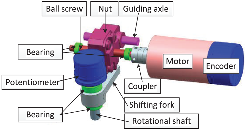
Structure of the EMA system.
Figure 2 shows the block diagram of double closed-loop control system for EMA system. TMS320F28335 DSP combined with CPLD is adopted to achieve one DSP controlling four channel EMA systems. DSP is utilized to implement sophisticated control strategies. CPLD is utilized to implement digital power converter control units. When command angular is given by the flight control system, DSP will analyze the command words and sensors signal to export pulse width modulation (PWM) control signal by angular position controller and angular velocity controller. Then, CPLD can capture hall signals and process them with PWM control signal. Thus, the control signal of EMA is obtained by CPLD and exports to EMA by PWM power driving circuit which consists of three-phase inverter and insulated gate bipolar transistor (IGBT) driver board. A cascade structure that consists of the speed loop and position loop is a classic way to control EMA system. Speed loop can reject the disturbances and improve rapidity of EMA system, thus it requires excellent steady state and dynamic performances. Position loop can make the aero fin follow the missile demand. In this article, a novel controller strategy is developed for speed loop to improve the performance of EMA system.

Block diagram of the double closed-loop control system for EMA system.
Mathematical model of EMA
The EMA system is driven by the brushless direct current motor (BLDCM) which is widely used since it ensures good control system performance in mechanical applications. The current equation and torque equation of BLDCM are shown in equations (1) and (2), respectively 9
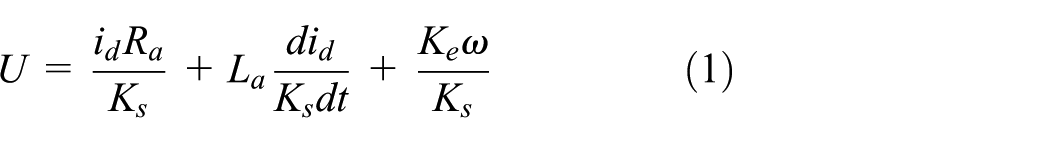

where
The dynamic model of EMA using Euler–Lagrange equation can be given as follows

where
The principal load torque of EMA is the hinge moment induced by aerodynamic forces on control surface which can lead to instability of missiles under certain condition. 52 The load torque can be expressed as

where
It can be concluded that hinge moment varies widely depending on specified flight condition and maneuvering status. The traditional way to obtain the approximate value of hinge moment coefficient is computational fluid dynamics, aerodynamic parameter identification, or wind tunnel experiments. 53 And then, the approximate maximum of hinge moment is calculated and is utilized to select BLDCM. However, the accurate value of hinge moment cannot be obtained. Thus, the variable load torque is considered as an external disturbance of the EMA system.
As a result, the state-space equation of EMA system including disturbances is shown in equation (5)

where
Assumption 1
According to the mechanical limitations of EMA, the angular position
Assumption 2
According to the limited of hardware, the control signal
Assumption 3
The nonlinear analysis of EMA system ignores the effect of elastic, and the mechanical structure is regarded as a rigid body.
Assumption 4
The angular position
In this article, the system disturbances can be divided into two parts. One is the model-based friction torque disturbance which can be identified by experiments, and the other is the residual disturbance which cannot be identified by experiments. The residual disturbance includes back electromotive forces, friction compensation error, variable hinge moment, and the model uncertainty.
Friction model
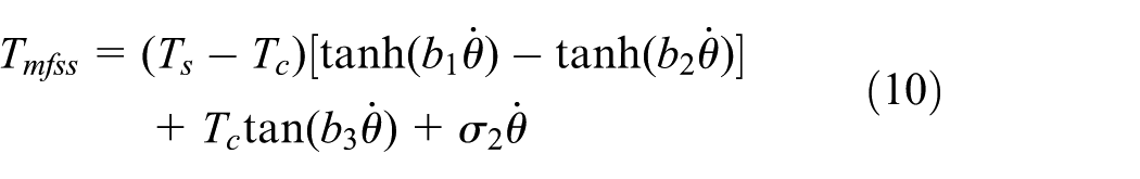
LuGre model is the syntheses of Danl model and Stribeck effect. Bristles are adopted to describe the contact surface and modeled by stiffness and damping. However, the model and its derivatives are discontinuous. Therefore, a continuous modified LuGre model is adopted. The model is proposed by J Yao et al. 20 and is based on hyperbolic tangent approximation instead of sign function in the LuGre model. The modified LuGre model avoids the discontinuity at the vicinity of zero angular velocity. It is described by


where
Several schemes are reported to identify the friction parameters of the friction model.54,55 The static parameters, such as

Replacing equation (9) in equation (6), the steady friction torque becomes
Combining equations (2) and (3),

where
Dynamic parameters are identified by model linearization at

Set

When the motion of the EMA system is at a small displacement and reaches a steady state, the equation (13) can be reduced to

The EMA system can be regarded as a mass-spring-damper system. Set

It can be implied from equation (15) that the friction behavior in the EMA system approximates to second-order damping system. As a result of this,
However, for a real system, due to the fact that EMA system is simplified to a second-order linear system, we can only get the ideal dynamic parameters in some ways. It is very difficult to get the accurate values; thus, an intelligent estimating scheme is also necessary.
EMA system control strategy
Figure 3 shows the block diagram of the controller structure for speed loop of the EMA system. The control strategy consists of ASMC, ESO, and friction compensation.

Block diagram of the proposed controller structure for speed loop of the EMA system.
ESO design
As shown in Figure 3, after friction compensation, equation (5) can be written as follows

where

Assumption 5
Function
Assumption 6
The functions
According to the ESO design method, 57 a second ESO is introduced as follows


The fitting schematic diagram of Fal function is shown in Figure 4. Figure 4 implies that the larger the error between the input and the output, the smaller the gain, the smaller the error between the input and the output, the larger the gain.52,58 Thus, Fal function has a linear zone output around the zero input. The Fal function is used to adjust the ESO gains by the error

Fitting schematic diagram of Fal function.
Here, the method of bandwidth–parameterization is applied to the ESO,27,50 thus
Unfortunately, if the ESO observer is not well selected, there always remains a non-null estimation error. The estimation error is defined as

where
The convergence of the ESO is given by and is omitted here.
53
The convergence can be achieved by choosing the parameters of
The main objective of ESO is to estimate the total disturbance in real time. However, although the high bandwidth of the parameters of ESO improves the disturbance rejecting ability, it will magnify sensor noise and dynamic uncertainties. So a trade-off between noise and rapidity should be made by trial and error.
Control law design
Based on the feedback control method shown in Figure 3, the control law

Sliding surface is selected generally as follows

where
The derivative of equation (21) is as follows

Combining equations (16) and (20) and substituting them into equation (22), we can obtain

We set

The nonlinear switching control to deal with the disturbance is given as
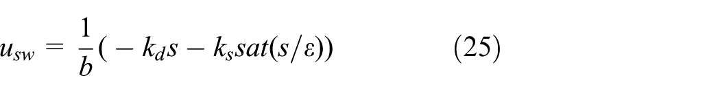
where
Analysis of stability
As we know, the upper bound of

Since

where
Theorem 1
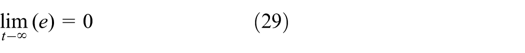
Considering the nonlinear system equation (5) under assumption 1–6 and sliding mode surface equation (21), for any initial states and desired reference angular velocity, the control laws in equation (26) and (28) for controlling EMA system are adopted to achieve the objective as follows
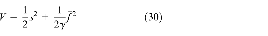
Define a positive-definite Lyapunov function for the closed-loop system
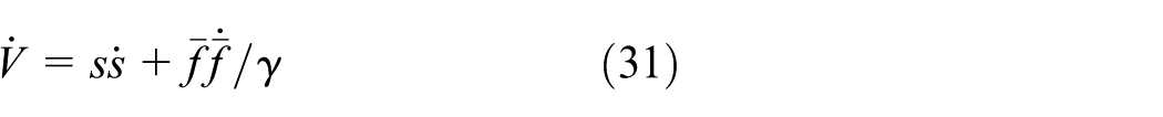
The time derivative of function V can be obtained as
Substituting equation (26) into equation (31), we obtain

Substituting equation (28) into equation (32), we obtain


Then, integrating the expression

Therefore, we have
As a result, the stability of closed dynamics can be guaranteed. Finally, the objective in equation (29) can be achieved.
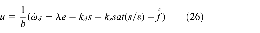
The final adopted control law is as follows

Equation (36) can be achieved by choosing the appropriate parameters
Experimental results
This section describes the experiments to validate the performance of the proposed control strategy. Since friction nonlinear and disturbance are the most important factors influencing the performance of EMA system, the experiments are mainly on these two aspects. Four experiments are carried out for the EMA system. The first experiment is used to identify the parameters of the friction model using constant angular velocity conditions. The second experiment is used to analyze the speed loop and validate the performance of the proposed control strategy. The third experiment is used to analyze the performance of double closed loop by step response and sinusoidal signal response. Due to the fact that the EMA system is a position tracking system which has a requirement for rapidity, the fourth experiment is used to validate the rapidity of the proposed control strategy.
Friction parameters identification
The experimental facility for friction identification is shown in Figure 5, which consists of a host PC, EMA system, target PC, power, frequency response analyzer, and a bench. The sampling time is 1 ms. The controllers are discretized by bilinear transformation and are carried out using TMS32028335 and CPLD. Meanwhile, Xpc target system is used to monitor the output of system by Controller Area Network (CAN) data acquisition board. The corresponding system parameters are specified in Table 1.

Experimental facility for friction identification of EMA system.
Parameters of the EMA system.

Based on the constant angular velocity conditions proposed in section “EMA system modeling,” an experimental test is carried out at different angular velocities ranging from ±10 to ±910 r/min with the interval of 50 r/min. Using the least square method, static parameters are obtained from Stribeck identification curve (Figure 6). The dynamic parameters are identified through eight experiments by double closed-loop control at different angular positions from ±0.05 degrees to ±0.2 degrees with the interval of 0.05 degrees. Static and dynamic parameters of the modified LuGre model are shown in Table 2.

Stribeck identification curve of EMA system.
Static and dynamic parameters of modified LuGre model.

Remark
The friction torque is the equivalent torque of the side of the motor. The friction torque of the side of output shaft is the product of this friction torque and the transmission rate.
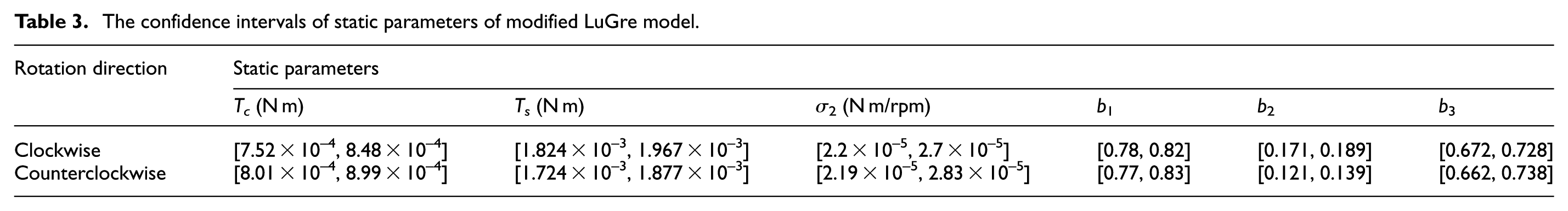
Due to the differences of the nonlinear factors and other disturbances between the positive and negative rotary directions, the parameters of the friction behavior of the two rotary directions are slightly different. A lot of repeatable experiments have been done for friction identification. Through experimental samples and statistical formulas, the confidence intervals of friction parameters are obtained and shown in Tables 3 and 4.
The confidence intervals of static parameters of modified LuGre model.
The confidence intervals of dynamic parameters of modified LuGre model.

Speed loop analysis
The system is a double closed-loop control system. The inner loop is the speed loop, and the outer loop is the position loop. According to the test principle, the speed loop is analyzed first. The experimental platform for speed loop performance test and position loop performance test is shown in Figure 7. It consists of EMA system, electric load simulator (ELS), and ELS control desk. The ELS is widely applied in missile industries. Here, ELS is used to simulate the load torque of the EMA system. As shown in Figure 7, the EMA system and ELS are connected mechanically by coupler, and the direction of the ELS is reverse to the rotational shaft.

Experimental platform of EMA system.
Based on the above analysis, the following three controllers of speed loop are compared on EMA system to validate the effectiveness of the proposed control strategy:
ASMC-ESO-MLuGre. This control strategy consists of ASMC, ESO, and friction compensation proposed above. The parameters of this controller through trial and error are
ASMC-MLuGre. This control strategy consists of ASMC and friction compensation proposed above. The controller parameters are
Proportional–integral (PI). The controller structure is shown below
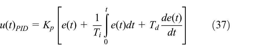
The proportional coefficient and the integral coefficient are considered as
The step reference curve of angular velocity at 1000 r/min is taken as a typical signal. Besides, it has torque disturbance using a sinusoidal signal with a magnitude of 3 N m and a frequency of 10 Hz from 0.3 to 0.6 s, a magnitude of 6 N m, and a frequency of 10 Hz from 0.6 to 1 s. The disturbance is produced by ELS. The step response is displayed in Figure 8. The disturbance rejecting ability is evaluated using standard deviation of tracking error. Table 5 shows the comparison of controller performance. Obviously, it is demonstrated that the ASMC-ESO-MLuGre shows a faster response, lower overshoot, and lower standard deviation with disturbance. It is seen that the performance of ASMC-ESO-MLuGre excels PI and ASMC-MLuGre.

Step response of angular velocity at 1000 r/min with disturbance by three kinds of controllers: (a) step response, (b) partial enlarged drawing from 0 to 0.3 s, and (c) partial enlarged drawing from 0.3 to1 s.
Comparison of controller.

PI: proportional integral; ASMC: adaptive sliding mode control; ESO: extended state observer.
Position loop analysis
PI controller is selected for the position loop, and the controller parameters by trial and error are as follows:
Disturbance rejecting ability analysis
The step response of angular position with the disturbance is shown in this section. In order to test the disturbance rejecting ability of the proposed control strategy, the disturbance torque produced by ELS is added into the system at 1 s. The disturbance torque is 5 N m. Transient response, disturbance rejection response, and steady-state response are depicted in Figure 9. The performance of the EMA system under different control strategies is shown in Table 6. It is obvious from Table 4 that the proposed control strategy provides better dynamic performance and steady-state performance and improves the disturbance rejecting ability.

Step response of angular position with disturbance.
Performance comparison of different controllers.

PI: proportional integral; ASMC: adaptive sliding mode control; ESO: extended state observer.
Small angular position tracking analysis
The sinusoidal instruction with amplitude 1 degree and frequency 1 Hz is taken as the reference angular position. Sinusoidal signal response of angular position at 1 sin (2πt) degree for each control method is shown in Figure 10. It is seen that when the angular velocity of the EMA system is close to zero, the PI controller cannot provide enough torque to support the nonlinear torque derived from nonlinear factors round the zero. The tracking curve becomes aberrant curve and produces zero-slip shown in Figure 10(a). Meanwhile, the position tracking curve produces stick-slip motion shown in Figure 10(b). However, the tracking curves adopting the friction compensation have a short time zero-slip of speed tracking curve and a short time stick-slip motion of position tracking curve. The tracking curves adopting the friction compensation and ESO have no zero-slip of speed tracking curve and no stick-slip motion of position tracking curve. It can be seen that the performance of proposed control strategy has the advantage over the other two controllers.

Sinusoidal reference trajectories of angular at 1 sin (1πt) degree: (a) angular velocity tracking curve and (b) angular position tracking curve.
Bandwidth test
Since the better disturbance rejecting ability of the proposed control strategy is validated above, it is needed to test the bandwidth of the EMA system which is a very important index. The experimental facility is shown in Figure 7 without load torque. Thus, no load is added when testing response bandwidth of the EMA system. The sweep signals produced by frequency response analyzer are taken as the demands reference signal of the EMA system. The magnitude of the sweep signals is 2 degrees, and the frequency is ranging from 0.7 to 27 Hz with the interval of 0.1 Hz. The response of the EMA system is analyzed by frequency response analyzer. Figure 11 shows the comparison of frequency response under the aforementioned three control strategies for double closed-loop EMA system. It depicts that the bandwidth is 22.82 Hz based on PI controller, 23.01 Hz based on ASMC-MLuGre, and 24.13 Hz based on the proposed controller. It can be concluded that the proposed controller excels the other two controllers.

Frequency response of double closed-loop system.
In a word, the experiments show that the proposed controller not only rejects disturbance and the effect of friction but also increases the static and dynamic performances of the EMA system.
Conclusion
In this article, a new control strategy composed of ASMC, ESO, and friction compensation is designed for the speed loop of EMA system to improve the performance. The disturbance of EMA system is divided into friction disturbance and residual disturbance. Friction torque is identified and compensated first. And then residual disturbance is estimated by ESO which does not depend on the information on model and compensated in the control action. ASMC is adopted to improve the performance of EMA system furthermore. The proposed control strategy is implemented on an experimental facility using step reference tracking of angular velocity with disturbance, step reference tracking of angular position with disturbance, sinusoidal reference tracking at small angular position, and frequency response analysis. According to the obtained results, it can be concluded that the proposed control strategy not only has better disturbance rejecting ability but also has better steady state and dynamic performance.
Besides, there is still a great deal research deserves to do in the future. Actually, we only compare the performances of each controller in its dynamic and static response performances, which is a conventional method to verify a new controller. Because an allowable maximum control input is set in the controller procedures of the three controllers to avoid damaging the EMA system, we do not test the control power for each controller. Indeed, the control power is also a comparison criterion of each controller. We should carry out research in this field in the future. The complexity of each controller is really different, and the most complex controller is the proposed controller. The parameters in this article are all debugged by trial and error method. The proposed controller needs to debug eight parameters, which increases debugging difficulty. An efficient automatic parameter debugging method is also needed to study in the future.
Footnotes
Handling Editor: Xiang Yu
Declaration of conflicting interests
The author(s) declared no potential conflicts of interest with respect to the research, authorship, and/or publication of this article.
Funding
The author(s) disclosed receipt of the following financial support for the research, authorship, and/or publication of this article: This work was supported by the 3rd Innovation Fund of Changchun Institute of Optics, Fine Mechanics and Physics (CIOMP).