Sage Journals: Discover world-class research

Abstract

Fault diagnosis for turnouts is crucial to the safety of railways. Existing studies on fault diagnosis depend on human experiences to select reference curves and require fault type information beforehand. Therefore, we proposed a turnout fault diagnosis method, named similarity function and fuzzy c-means based two-stage algorithm to detect faults and identify fault types in real time. First, the reference curve is selected from current curves representing turnout actions by K-means algorithm; then, a similarity function called Fréchet distance is used to distinguish normal and abnormal curves. Second, an improved fuzzy c-means algorithm is employed to cluster curves automatically. To be more specific, it can double-confirm the normal curves recognized in the first step as well as divide the abnormal curves into different types. Furthermore, possible causes for each fault type are inferred according to their curves. Our approach integrates fault detection and fault classification into one model and would better help the diagnosis of turnouts. The analysis results based on the similarity function and fuzzy c-means based two-stage algorithm algorithm indicate that the analyzed turnout fault types can be diagnosed automatically with high accuracy. Furthermore, since the proposed similarity function and fuzzy c-means algorithm does not need to know fault types in advance, it is applicable in identifying new fault types.

Keywords

Turnout fault diagnosis Fréchet distance fuzzy c-means algorithm similarity function and fuzzy c-means based two-stage algorithm

Introduction

High-speed railway (HSR) has developed rapidly in China over the past several years,¹ and the operation and maintenance departments of HSR have faced an increasing requirement for transportation safety monitoring.² Meanwhile, many monitoring systems have put the emphasis on the reliability of turnouts³ because turnouts are a crucial part for the safety of a whole railway network and⁴ they are easier to be broken. First of all, the blades of turnouts hold a much weaker mechanical strength than regular rails do, and their mechanical properties are more likely to change. Any tiny transformation of blades might result in excessive forces on turning points or even derail a train. Second, turnouts are exposed in complex environments and unexpected accidents might happen, e.g., blades being stuck. Thus, the normal operation of the turnout is still a challenge.

A typical railway signal monitoring system works in two steps: first, it captures current values, which are produced by turnout movements, with an interval of 40 ms; second, it shows the captured current values in a current-time plane, which using time as the horizontal axis and current values as vertical axis.⁵ Therefore, the curves can help to analyze turnout actions and attract most studies on fault diagnosis.^6–8

Technically, fault diagnosis is different from fault detection. The former is not only to identify irregularities/faults from normalcies, but also to sort out different types of faults, while the latter is only to identify faults. Intelligent fault detections and diagnoses for turnouts have attracted many researchers. Huang et al.⁹ developed an intelligent diagnosis method for railway turnout using dynamic time warping. Atamuradov et al.¹⁰ utilized expert systems to conduct turnout fault diagnosis. Wang et al.¹¹ presented a failure prediction model based on Bayesian network to evaluate the effect of weather on railway turnouts. Vileiniskis et al.¹² presented a one-class support vector machine classification to predict possible failures in the system. Asada and Roberts¹³ utilized wavelet transforms and support vector machines to realize turnout fault detection and diagnosis. Kim et al.¹⁴ proposed a fault detection method based on dynamic time warping for railway point machines. Ross¹⁵ designed a monofocal camera–based fault detection for turnouts. J Lee et al.¹⁶ presented a data mining solution that utilized audio data to efficiently detect and diagnose railway faults. Zhao et al.¹⁷ applied gray theory to turnout fault diagnosis.

Although the above studies are elegant, there is still some room for improvement. First of all, they all require a training set with labels and known curves as well as failure types as references.¹⁸ However, all the labels, the optimal reference curves and reasonable fault types are determined based on human experiences, which means the accuracy of fault diagnosis has to entirely depend on the most unstable and complicated factor. Furthermore, turnout actions are affected by complex factors, like locations, weather, and working hours; therefore, its normal actions are not fixed and may slightly change, and new types of faults may emerge. Nevertheless, the above research cannot update their reference curves and fault types in real time. Third, when a new fault type emerges, chances are high that it cannot be recognized if a reference curve has not been known beforehand.

Therefore, we present similarity function and fuzzy c-means based two-stage (SF-FCM-TS) algorithm, a fault diagnosis method, to select the reference curves independently from human aid and to identify new fault types without prior information.

Methodology

SF-FCM-TS consists of two stages: fault detection and then clustering and verification. Fault detection in SF-FCM-TS works in this way: first, the reference curve is selected by K-means algorithm from a bunch of none-label curves, which were obtained from field turnout action monitoring systems. Second, the similarity between sample curves and the reference curve is calculated based on the Fréchet distance. Finally, a reasonable threshold for fault is determined.

In the second stage, an improved fuzzy c-means (FCM) algorithm is proposed to cluster sample curves automatically and identify fault types. Furthermore, it verifies the selection of the reference curve and the accuracy of fault detection in the first stage.

These two stages are integrated into one model and the second stage also serves as a double check for the first stage. Sample curves are divided into the normal and the abnormal categories in the first stage. In the second stage, the normal ones are confirmed and the abnormal ones are divided into different types. The workflow of the proposed approach is shown in Figure 1.

Figure 1.

Similarity function and fuzzy c-means based two-stage algorithm.

The first stage—fault detection

Since turnouts work normally most of the time, we assume that the majority of curves of a certain turnout are normal within a certain period of time. Fault detection in SF-FCM-TS includes three steps: selecting a reference curve, calculating similarities, and determining fault threshold.

Selecting reference curve

Three steps are designated to ensure the final selected reference curve is representative and standard: pretreatment, point analysis, and line analysis.

Pretreatment

Pretreatment is to select those curves which contain the highest number of repetitious sampling time points.

The set of original test curves consists of n curves denoted as

L' = [{l'}_{1}, {l'}_{2}, \dots, {l'}_{n'}]

(1)

H = [h_{1}, h_{2}, \dots, h_{n'}]

(2)

H is the number of sampling time points of each curve in $L'$ and $h_{i}$ is the number of sampling time points of $l'_{i} (i \in [1, n'])$ .

U represents the highest repetition number in H. If $h_{i}$ is not equal to U, $l'_{i}$ is removed from $L'$ . Therefore, the set of final sample curves are denoted as

L = [l_{1}, l_{2}, \dots, l_{n}]

(3)

Point analysis

Point analysis aims to obtain the clustering center of each sampling time point by K-means algorithm.

The current value of each sampling time point is denoted as C

C = [\begin{matrix} l_{1} \\ ⋮ \\ l_{n} \end{matrix}] = [\begin{matrix} c_{11} & \dots & c_{1 U} \\ ⋮ & c_{ij} & ⋮ \\ c_{n 1} & \dots & c_{nU} \end{matrix}]

(4)

where $c_{ij} (i \in [1, n], j \in [1, U])$ is the current value of the jth sampling time point of the ith curve.

The set of sampling time points is denoted as

P = [p_{1}, p_{2}, \dots, p_{U}]

(5)

And the set of the jth sampling time point $p_{j} (j \in [1, U])$ is

p_{j} = {(c_{1 j}, c_{2 j}, \dots, c_{nj})}^{'}

(6)

Then, the clustering centers of sampling time points are denoted as

Z = [z_{1}, z_{2}, \dots, z_{U}]

(7)

where $z_{j} (j \in [1, U])$ is the clustering center of the jth sampling time point. $z_{j}$ can be calculated by K-means algorithm¹⁹

z_{j} = K - means (p_{j})

(8)

Figure 2 illustrates how to obtain clustering center $z_{j}$ of the jth sampling time point.

Figure 2.

Process of obtaining clustering center $z_{j}$ of the jth sampling point.

Then, the intervals of the clustering centers can be denoted as

I = [i_{1}, i_{2}, \dots, i_{U}]

(9)

where $i_{j} (j \in [1, U])$ is the interval of the jth clustering center and calculated through

i_{j} = [z_{j} - e, z_{j} + e]

(10)

where $e$ is the interval radius, set based on actual condition and human experiences.

Line analysis

Line analysis is to figure out the number of clustering centers involved in each curve, therefore to identify the representation for each curve.

Suppose curve l_i is

l_{i} = [c_{i 1}, c_{i 2}, \dots, c_{iU}]

(11)

where $c_{ij} (j \in [1, U])$ is a point in l_i . If $c_{ij} \in i_{j}$ , $c_{ij}$ is a clustering center. Then, the number of clustering centers involved in each curve is denoted as

M = [m_{1}, m_{2}, \dots, m_{n}]

(12)

where $m_{i} (i \in [1, n])$ is the number of clustering centers involved in the ith curve. $m_{\max}$ is the maximum value of M. If $m_{k} = m_{\max}$ and $k \in [1, n]$ , the kth curve is identified as the reference curve $l_{r}$ .

Calculating similarity

The Fréchet distance

Distance space, also known as the Fréchet distance, is first proposed by Maurice Fréchet, a French mathematician, in 1906. It extends the concept of distance in real world to general set, providing a theoretical base for measuring distances between abstract spaces.

Suppose

f : I = [l_{I}, r_{I}] \to R^{2}

(13)

and

g : J = [l_{J}, r_{J}] \to R^{2}

(14)

are two planar curves, and ∥·∥ the Euclidean norm. Then the Fréchet distance $δ_{F} (L_{1}, L_{2})$ is defined as

δ_{F} (L_{1}, L_{2}) = \inf_{\binom{α : [0, 1] \to I}{β : [0, 1] \to J}} \max_{t \in [0, 1]} ‖ f (α (t)) - g (β (t)) ‖

(15)

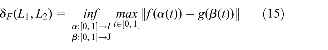
where $α$ and $β$ range over continuous and non-decreasing reparametrizations with $α (0) = l_{I}$ , $α (1) = r_{I}, β (0) = l_{J}, β (0) = l_{J}$ .

We adopt the discrete Fréchet distance, for the convenience of digital processing. Thus, the distance between curves $l_{1}$ and $l_{2}$ is calculated as follows:

Step 1: The first curve $l_{1}$ is described as

P = {P (1), P (2), \dots, P (n), \dots, P (N)}

(16)

P (n) = (x_{n}, y_{n})

(17)

where n is the number of the sampling points and $n \in [1, N]$ ; $x_{n}$ the abscissa of the nth sampling point; and $y_{n}$ the ordinate of the nth sampling point.

Step 2: The second $l_{2}$ is presented as

P' = {P' (1), P' (2), \dots, P' (m), \dots, P' (M)}

(18)

P' (m) = ({x'}_{m}, {y'}_{m})

(19)

where m is the number of the sampling points and $m \in [1, N]$ ; $x'_{m}$ the abscissa of the mth sampling point; and $y'_{m}$ the ordinate of the mth sampling point.

Step 3: The Euclidean distance D between the sampling points $L_{1}$ and $L_{2}$ is calculated as

D = [\begin{matrix} d_{11} & \dots & d_{1 N} \\ ⋮ & d_{mn} & ⋮ \\ d_{M 1} & \dots & d_{MN} \end{matrix}]

(20)

where $1 \leq m \leq M, 1 \leq n \leq N$ ; and

d_{mn} = \sqrt{{({x'}_{m} - x_{n})}^{2} + {({y'}_{m} - y_{n})}^{2}}

(21)

is the Euclidean distance between the mth sampling point of $L_{1}$ and the nth sampling point of $L_{2}$ .

Step 4: The maximum value of D is denoted as $d_{\max} = \max (D)$ , while the minimum value of D is denoted as $d_{\min} = \min (D)$ . Then, the initial target distance f is set as $f = d_{\min}$ and the cycle interval res is

res = \frac{d_{max} - d_{min}}{100}

(22)

Step 5: In equation (20), if $d_{mn} \leq f$ , then $d'_{mn} = 1$ ; if $d_{mn} > f$ , then $d'_{mn} = 0$ . Therefore, the binary matrix $D'$ can be described as

D' = [\begin{matrix} {d'}_{11} & \dots & {d'}_{1 N} \\ ⋮ & {d'}_{mn} & ⋮ \\ {d'}_{M 1} & \dots & {d'}_{MN} \end{matrix}], d'_{mn} = {\begin{matrix} 1, {d'}_{mn} \leq f \\ 2, {d'}_{mn} > f \end{matrix}

(23)

where $1 \leq m \leq M and 1 \leq n \leq N$ .

Step 6: A set

R = [{d'}_{11}, \dots, {d'}_{mn}, \dots, {d'}_{MN}]

(24)

is constructed with the limit of

d'_{11} \times \dots \times d'_{mn} \times d'_{(m + k) (n + k')} \times \dots \times d'_{MN} = 1

(25)

where $1 \leq m \leq M, 1 \leq n \leq N, 1 \leq m + k \leq M, 1 \leq n + k \leq N, k = {0, 1}, k' = {0, 1}$ .

Step 7: If the construction of R fails, let $f = f + res$ and repeat steps 5 and 6. If a set R is built or $f = d_{\max}$ , proceed to the next step.

Step 8: The discrete Fréchet distance between $l_{1}$ and $l_{2}$ is

Frechet (l_{1}, l_{2}) = f

(26)

Similarity between normal curves and the reference curve

$S (l_{1}, l_{2})$ is the similarity between $l_{1}$ and $l_{2}$ and calculated as

S (l_{1}, l_{2}) = \frac{1}{Frechet (l_{1}, l_{2})}

(27)

Therefore, the similarity between the sample curves and the reference curve $l_{r}$ can be described as

S = [s_{1}, s_{2}, \dots, s_{n}]

(28)

where $s_{i} (i \in [1, n])$ is the similarity between the ith curve and the reference curve and calculated by equation (27).

Determining threshold

Few fault curves may still stay in the sample curves and each of them may contain the same number of sampling points as the reference curve does. However, these possible fault curves are far less similar with the reference curve than other normal curves. Therefore, the especially small ones in S are removed, and the minimum of the rest is denoted as $s_{\min}$ . Then the threshold $s_{t}$ can be calculated as

s_{t} = k \times s_{min}

(29)

where k is the adjustment factor set based on actual condition. Here, we set k as 0.95.

The threshold $s_{t}$ is used to judge whether a turnout fails. If the similarity between a certain curve and the reference curve is smaller than $s_{t}$ , the turnout which the curve represents must have something wrong. If the similarity is larger than $s_{t}$ , the turnout works well.

The second stage—clustering and verification

Data preprocessing

Data preprocessing includes data normalization and data dimensionality reduction. Since different turnouts’ movements may last differently, curve lengths are different, and a single curve may contain hundreds of data points, leading to a large data dimension and poor clustering results. Therefore, the original data need to be normalized so that each curve could contain the same number of data points. The normalization is performed as follows:

Step 1: Construct H as described in equation (2). And assign each curve a vector of its data, that is, N curves, N vectors.

Step 2: Compare each $h_{x}$ in H with a specified number, set as 200 in this article. If $h_{x}$ is smaller than the number, each element of the corresponding vector is set as zero; while if $h_{x}$ is larger, the corresponding vector is compressed to contain the specified number of elements.

Step 3: Subtract the average of a certain curve from each data value in the curve.

After normalization, principal component analysis (PCA) is used to reduce the dimension.

FCM algorithm

Fuzzy c-means (FCM) algorithm is a kind of cluster analysis. Cluster analysis, or clustering, is the process of categorizing a set of objects so that objects in the same category, or cluster, are more similar in certain aspects to each other than to those in other clusters. Clustering is known as unsupervised learning since no labeling information is required.

FCM algorithm was developed by JC Dunn²⁰ and improved by JC Bezdek.²¹ The basic idea of FCM algorithm is to update the clustering center and membership degree matrix repeatedly²² until the objective function achieves the minimum value. Thus, the data classification is completed based on the maximum membership degree principle.

FCM aims to minimize an objective function²³

J_{m} (U, V) = \sum_{j = 1}^{n} \sum_{i = 1}^{c} u_{ij}^{m} d_{ij}^{2} (x_{j}, c_{i})

(30)

where m is any real number greater than 1 and usually set as 2; $u_{ij}$ the degree of membership of $x_{j}$ in cluster i; c the number of clusters; $x_{j}$ the jth of d-dimensional sample; $c_{i}$ the d-dimensional center of the cluster; N the number of samples and $d_{ij}$ the Euclidean distance between any sample j and the center i.

Equation (30) is constrained by

{\begin{matrix} \sum_{j = 1}^{c} u_{ij} = 1, 1 \leq j \leq n \\ 0 \leq u_{ij} \leq 1, i = 1, 2, \dots, n \\ 0 < \sum_{j = 1}^{n} u_{ij} < n, 1 \leq i \leq c \end{matrix}

(31)

Equation (31) is substituted into equation (30) by Lagrange multiplier method and then the partial derivative is calculated. The cluster center $c_{i}$ is computed by

c_{i} = \frac{\sum_{j = 1}^{n} u_{ij}^{m} x_{j}}{\sum_{j = 1}^{n} u_{ij}^{m}}

(32)

The $u_{ij}$ is calculated by

u_{ij} = \frac{1}{\sum_{k = 1}^{c} {(\frac{d_{ij}}{d_{kj}})}^{\frac{2}{m - 1}}}

(33)

The FCM algorithm follows next steps:

Step 1: Determine the number of the clusters (c). Initialize m, $U^{(i)} = matrix$ , and $U^{(0)}$ .

Step 2: At i-step, calculate $c_{j}$ with $U^{(i)}$ by equation (32).

Step 3: Update $U^{(i)}$ to $U^{(i + 1)}$ by equation (33).

Step 4: If $‖ U^{(i + 1)} - U^{(i)} ‖ < ε$ , then stop; otherwise return to Step 2.

Improved FCM algorithm

Basic FCM algorithm cannot determine the number of the clusters automatically. Therefore, Silhouette_Score (SS), the mean Silhouette Coefficient of all samples, is adopted to measure the clustering effects. The Silhouette_Score for each sample is calculated as

silhouette_score = \frac{b - a}{max (a, b)}

(34)

where a is the mean intra-cluster distance and b the mean nearest-cluster distance,²⁴ a distance between a sample and its nearest neighbor cluster. The larger the value of SS, the better the clustering effect. Therefore, when SS achieves max, the corresponding number of clusters is the optimal. Figure 3 illustrates the workflow of finding the optimal number using the improved FCM algorithm.

Figure 3.

Improved FCM algorithm flowchart.

Verification and classification

The second stage involves Verification and Classification.

First, the normal curves selected in the first stage are clustered by FCM algorithm. If they all fall into the same cluster, that is, they are all normal; the reference curve selected in the first stage is verified.

Second, the abnormal curves classified in the first stage are also clustered by FCM algorithm, and different types of faults can be obtained. And the reason for each type of fault can be analyzed consequently.

Application

Testing data

We chose ZD6 turnout’s data for our application and validation of the proposed methodology, considering its wide application. And the turnout’s data were gleaned in the Jinan Railway Station from 12 December 2017 to 10 January 2018. It is a total of 817 curves of four turnouts.

Testing results

We selected 70% of the 817 curves gleaned in the Jinan Railway Station from 12 December 2017 to 10 January 2018, that is 572, as test curves and kept the rest 30% for verification. We used MATLAB 2014 to implement the application in first stage and we used python 3.5 to implement the application in second stage.

Fault detection

First, we conducted pretreatment on the test curves and obtained the distribution of the number of sampling time points of each curve, as shown in Figure 4. The most repetitious number of sampling time points was 236. Thus, we selected 109 curves for test form the total sample, whose sample size was 236. The rest curves were used for later analysis.

Figure 4.

Distribution of the number of sampling points.

Second, we utilized the K-means algorithm to calculate clustering centers of each of the 236 sampling time point. For example, the clustering center of the 15th sampling time point was 1.949, as the interval radius $e$ was set as 0.03.

Then we counted the number of clustering centers of each sample curve, as exhibited in Figure 5. The 52-th curve held the largest number of clustering centers, 75, which means the 52-th curve was the most representative and selected as the reference curve.

Figure 5.

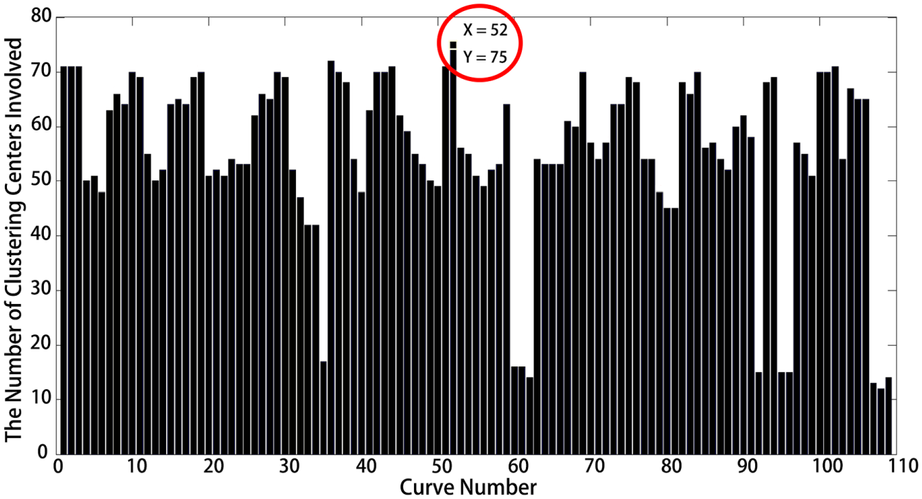
Number of clustering centers included in each curve.

Figure 6 depicts the reference curve, that is, the 52-th curve.

Figure 6.

Reference curve.

The reference curve can be split into four phases²⁵ according to typical movements of turnouts:

Unlocking (t0–t1): motor starts with large current value and torque, and the current rises rapidly.

Conversion (t1–t2): the turnout moves smoothly, and so does the current.

Locking (t2–t3): the switch rail moves to the other side until it is close enough to the stock rail when the current reduces to zero.

Slow-releasing (t3–t4): the relay releases slowly and the current remains zero.

Third, there were 108 sample curves, except the 52-th reference curve. And we calculated the similarity between each individual sample curve and the reference curve, based on the Fréchet distance, as shown in Figure 7. All the similarities fell within the range of [3.8, 4.1] and the minimum similarity $s_{\min}$ was 3.81. As the adjustment factor k was 0.95, we obtained the threshold $s_{t}$

s_{t} = k \times s_{\min} = 0.95 \times 3.81 = 3.6195

(34)

Figure 7.

Similarity between the normal curves and the reference curve.

Finally, we calculated the similarity between the reference curve and each individual of the total 571 test curves, including 108 sample curves, and compared each result with the threshold $s_{t}$ . If the similarity was below the threshold, the corresponding curve was determined to be abnormal. Therefore, we got 514 normal curves and 58 abnormal curves.

Fault diagnosis

Classification Step

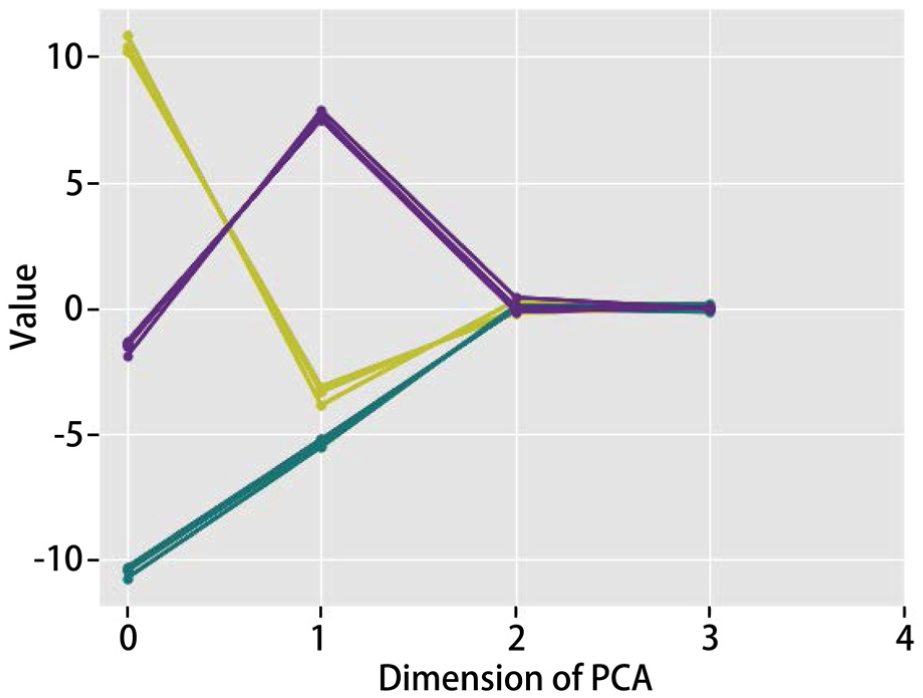
First, we normalized the dimension of each abnormal curves selected in the first stage as 200 and reduced it to 4 using PCA. The whole process is illustrated in Figure 8.

Figure 8.

Normalization and reduction of curve’s dimension.

Second, we run the loop function shown in Figure 3 to find the optimal number of clusters. As shown in Figure 9, SS first dropped when k changed to 4; thus, the optimal number was set as 3.

Figure 9.

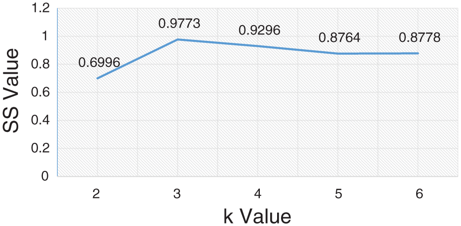
Value of SS (Classification Step).

Then we obtained the results of clustering curves (Figure 10) and their corresponding original ones (Figure 11).

Figure 10.

Clustering results (Classification Step).

Figure 11.

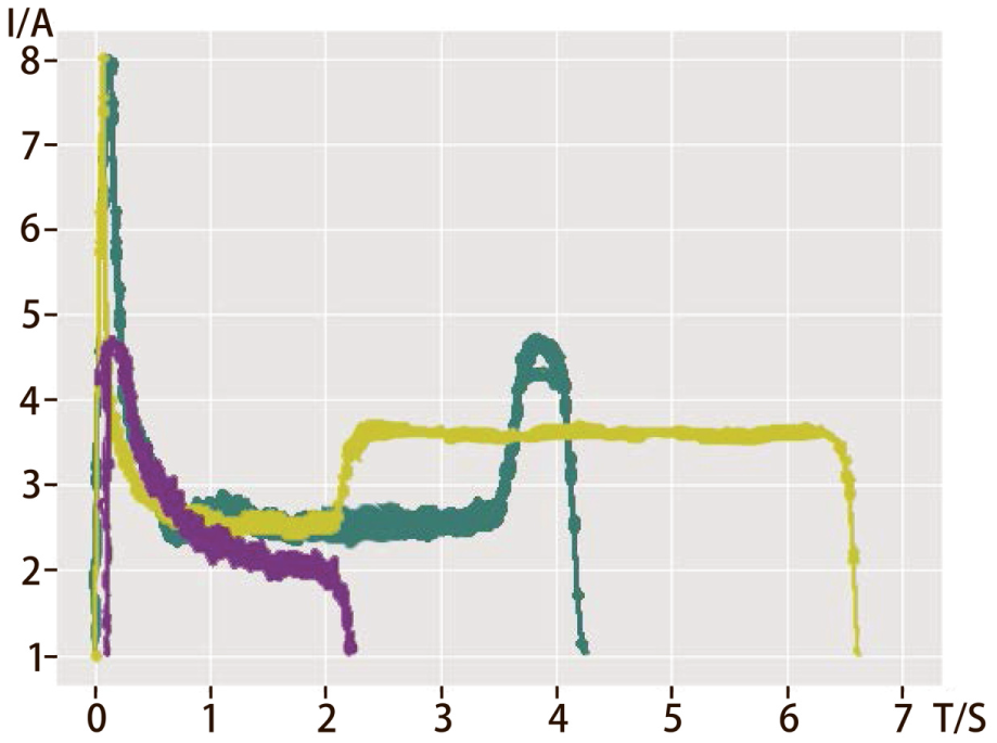
Corresponding curves of the clustering results (Classification Step).

These clusters, type green, type yellow, and type purple, were determined to be abnormal, but each of them held its unique feature, as analyzed below:

1. Type GREEN

In Type GREEN curve (Figure 12), the current rises sharply in the locking stage, possibly caused by an excessively tight turnout.

Figure 12.

Type GREEN curve.

2. Type YELLOW

Type YELLOW curve exhibits a longer locking line and higher current values, as depicted in Figure 13, possibly because that the automatic actuator is not flexible.

Figure 13.

Type YELLOW curve.

3. Type PURPLE

In Type PURPLE curve, the conversion time lasts shorter and the locking line does not even exist, as shown in Figure 14. The reason may lie in a sudden stop of the turnout’s movement.

Figure 14.

Type PURPLE curve.

Verification Step

Considering that the value of SS cannot be calculated when k = 1, we added a default set of curves in Verification Step. In this default set of curves, each curve has 200 sampling time points and the value of each sampling time points is −1. Obviously, when the normal curves and the default curves were clustered by FCM algorithm, if the number of clusters is two and only the normal curves selected in the first stage all fall into the same cluster, that is, they are all normal, the normal curves selected in the first stage is verified.

First, as Classification Step, we normalized the dimension of each normal curves and the default curves as 200, and reduced it to 4 using PCA. Second, we run the loop function shown in Figure 3 to find the optimal number of clusters. As shown in Figure 15, SS has been decreasing from k = 2 to k = 5; thus, the optimal number of clusters was set as 2.

Figure 15.

Value of SS (Verification Step).

Then, we obtained the results of clustering curves (Figure 16) and the corresponding original normal curves, the Type ORANGE curves (Figure 17).

Figure 16.

Clustering results (Verification Step).

Figure 17.

Type ORANGE curve.

Finally, by contrast, we found that the number and the serial number of each Type ORANGE curves obtained by our fault diagnosis method in Classification Step were exactly the same as those obtained by our fault detection method, which verified the reasonability of the reference curve and the accuracy of the previous fault detection.

Verification

We also calculated the similarity between the reference curve and each of the left 245 curves, 30% of the original 817 curves gleaned in the Jinan Railway Station from 12 December 2017 to 10 January 2018, and got 216 normal ones and 29 abnormal ones.

Then we clustered the 216 normal curves using the reference curve and the results indicated that all of them belonged to the same cluster, which verified the accuracy of the previous fault detection.

Finally, we clustered the 29 abnormal curves using the central curves of the three types of fault curves and obtained 13 of type green, 10 of type yellow, and 9 of type purple, which was also identical to the fault type in test samples.

Furthermore, our fault diagnosis method can identify new type of fault, when the number of clusters grows during clustering. And it can be applied to a real-time fault diagnosis system. For example, if a single curve is input, it will be added to the test curves and processed with them throughout the complete workflow.

Results and discussions

Finally, we got a bunch of normal curves and three types of fault curves. Not surprisingly, the similarity between each of the normal curve and the reference curve was larger than the threshold $s_{t}$ , while the similarity between each of the fault curve and the reference curve was much smaller than $s_{t}$ , which means the reference curve and the threshold $s_{t}$ can distinguish normal and abnormal curves without any mistake, thus verifies our approach. The results of 100% correct fault clustering and identification demonstrate high accuracy of our approach.

Moreover, the results imply other advantages of our SF-FCM-TS. First of all, fault type does not need to be known in advance. Second, new type of fault can be identified along with fault classification and diagnosis.

Conclusion

In this study, we proposed a turnout fault diagnosis method named SF-FCM-TS algorithm based on similarity function and improved FCM algorithm. The approach works in two stages. First, it automatically selects a reference curve and cluster abnormal curves based on the similarity of curve features. Second, it utilizes the improved FCM algorithm to verify the reasonability of the selection of the reference curve and the accuracy of fault detection in the first stage.

Our approach is independent from human experiences and can determine reference curve and fault types in real time. Even if the turnout action current curve changes slightly with location, weather, and working hours, the turnout fault can still be diagnosed. Also, the accuracy of fault detection is double-checked in the second stage, which will further enhance the safety of railway operation.

The proposed method can identify new fault types along with the clustering. And the introduction of Silhouette_Score to the fundamental FCM can directly provide the number of clusters. Therefore, our approach is fairly effective.

Furthermore, the proposed method is applicable to all types of turnouts as long as the action curves of the turnout can be obtained. Therefore, the applicability of this method is good.

We will focus on increasing effectiveness by trying other algorithms to define the similarity and by improving the FCM algorithm. In addition, we are exploring the robustness evaluation of the proposed method when weather or other transient conditions change.

Footnotes

Acknowledgements

The authors are grateful for the reviewers’ helpful comments and suggestions.

Handling Editor: Sunday Ojolo

Declaration of conflicting interests

The author(s) declared no potential conflicts of interest with respect to the research, authorship, and/or publication of this article.

Funding

The author(s) disclosed receipt of the following financial support for the research, authorship, and/or publication of this article: This research is supported by the National Key R&D Program of China (2016YFB1200402) and the National Natural Science Foundation of China (61703308).

ORCID iDs

Shize Huang

Ling Wang

References

Lin

Wang

et al . Inventory-transportation integrated optimization for maintenance spare parts of high-speed trains. PLoS ONE 2017; 12: e0176961.

Wang

. A New Early Warning Method of Train Tracking Interval Based on CTC. IEEE Transactions on Intelligent Transportation Systems 2012: 1524–9050.

Morant

Larsson-Kråik

Kumar

Data-driven model for maintenance decision support: a case study of railway signalling systems. Proc IMechE, Part F: J Rail & Rapid Transit 2016; 230: 220–234.

Gigante-Barrera

Dindar

Kaewunruen

et al . LOD BIM element specification for railway turnout systems risk mitigation using the information delivery manual. Mater Sci Eng 2017; 245: 042022.

Marugan

Marquez

FPG

. A novel approach to diagnostic and prognostic evaluations applied to railways: a real case study. Proc IMechE, Part F: J Rail & Rapid Transit 2016; 230: 1440–1456.

Zhou

Xia

Dong

et al . Fault diagnosis of high-speed railway turnout based on support vector machine. In: Proceedings of the international conference on industrial technology, Taipei, Taiwan, 14–17 March 2016, pp.1539–1544. New York: IEEE.

Zhang

. The railway turnout fault diagnosis algorithm based on BP neural network. In: Proceedings of the international conference on control science and systems engineering, Yantai, China, 29–30 December 2014, pp.135–138. New York: IEEE.

Zhang

. Algorithm of railway turnout fault detection based on PNN neural network. In: Proceedings of the 7th international symposium on computational intelligence and design, Hangzhou, China, 13–14 December 2014, pp.544–547. New York: IEEE.

Huang

Zhang

et al . Turnout fault diagnosis through dynamic time warping and signal normalization. J Adv Transp 2017; 2017: 1–8.

10.

Atamuradov

Camci

Baskan

et al . Failure diagnostics for railway point machines using expert systems. In: Proceedings of the international symposium on diagnostics for electric machines, power electronics and drives, Cargese, 31 August–3 September 2009, pp.1–5. New York: IEEE.

11.

Wang

Tang

et al . A Bayesian network model for prediction of weather-related failures in railway turnout systems. Expert Syst Appl 2016; 69: 247–256.

12.

Vileiniskis

Remenyte-Prescott

Rama

A fault detection method for railway point systems. Proc IMechE, Part F: J Rail & Rapid Transit 2016; 230: 852–865.

13.

Asada

Roberts

Improving the dependability of DC point machines with a novel condition monitoring system. Proc IMechE, Part F: J Rail & Rapid Transit 2013; 227: 322–332.

14.

Kim

Chung

et al . Fault diagnosis of railway point machines using dynamic time warping. Electron Lett 2016; 52: 818–819.

15.

Ross

Track and turnout detection in video-signals using probabilistic spline curves. In: Proceedings of the international conference on intelligent transportation systems, Anchorage, AK, 16–19 September 2012, vol. 24, pp.294–299. New York: IEEE.

16.

Lee

Choi

Park

et al . Fault detection and diagnosis of railway point machines by sound analysis. Sensors 2016; 16: 549.

17.

Zhao

Method of turnout fault diagnosis based on grey correlation analysis. J Chin Railw Soc 2014; 36: 69–74.

18.

Ponulak

Kasiński

Supervised learning in spiking neural networks with resume: sequence learning, classification, and spike shifting. Neural Comput 2010; 22: 467–510.

19.

Yang

et al . Optimization study on k value of k-means algorithm. Syst Eng Theor Pract 2006; 26: 97–101.

20.

Dunn

JC.

A fuzzy relative of the ISODATA process and its use in detecting compact well-separated clusters. J Cybernetics 1973; 3: 32–57.

21.

Bezdek

JC.

Pattern recognition with fuzzy objective function algorithms. New York: Plenum Press, 1981.

22.

Cai

Chen

Zhang

Fast and robust fuzzy c-means clustering algorithms incorporating local information for image segmentation. Pattern Recogn 2007; 40: 825–838.

23.

Liu

Wang

et al . A spacecraft electrical characteristics multi-label classification method based on off-line FCM clustering and on-line WPSVM. PLoS ONE 2015; 10: e0140395.

24.

Chang

Dai

Chen

CC.

A novel procedure for multimodel development using the grey silhouette coefficient for small-data-set forecasting. J Oper Res Soc 2015; 66: 1887–1894.

25.

Ren

Analysis of switch action status cures of micro-computer monitoring system. Railw Signal Commun 2009; 45: 36–37.

Two-stage turnout fault diagnosis based on similarity function and fuzzy c-means

Abstract

Keywords

Introduction

Methodology

The first stage—fault detection

Selecting reference curve

Pretreatment

Point analysis

Line analysis

Calculating similarity

The Fréchet distance

Similarity between normal curves and the reference curve

Determining threshold

The second stage—clustering and verification

Data preprocessing

FCM algorithm

Improved FCM algorithm

Verification and classification

Application

Testing data

Testing results

Fault detection

Fault diagnosis

Classification Step

Verification Step

Verification

Results and discussions

Conclusion

Footnotes

Acknowledgements

Declaration of conflicting interests

Funding

ORCID iDs

References