Sage Journals: Discover world-class research

Abstract

Wax deposition occurs frequently in waxy crude oil pipelines when the level of flow decreases, and pigging is needed at regular intervals. An economic pigging model is established in accordance with the objective function based on the sum of thermal costs, power costs, and single piping costs. Thus, by compiling a program, the most economical pigging cycle will be determined. Furthermore, the calculation methods for hydraulic and thermal constraints are given. Taking the example of the distance between the central processing platform and the land terminal external piping line of the M-field cluster, the effects of different inlet temperatures, throughput, and remnant wax thicknesses on the economic pigging cycle will be analyzed. The results show that with an increase in the inlet temperature, the total costs of the pipeline operation increase, while the pigging cycle will prolong. As throughput increases, total costs will decrease, while the pigging cycle also extends. When throughput is fixed, a remnant wax thickness of 0.4 mm helps reduce the total operating costs of the pipeline at different inlet temperatures. While throughput varies, a remnant wax thickness from 0.2 to 0.4 mm can reduce total costs at a fixed inlet temperature.

Keywords

Waxy crude oil pipelines low throughput pigging cycle the nature of economy remnant wax thickness

Introduction

According to incomplete statistics, China National Offshore Oil Corporation has laid 315 submarine pipelines (with diameters from 50.8 to 762.0 mm) in China’s seas, with a combined length of approximately 6202 km.¹ As submarine pipelines are buried deep under or flatly laid on the seabed, the factors that should be taken into consideration to design, operate, and maintain them are clearly different from those for terrestrial pipelines. Until now, domestic crude oil was generally manufactured in low volumes and had a high wax content, high freezing point, and high viscosity; consequently, the fluidity of crude oil was poor.² Owing to the low temperature on the seabed, the temperature quickly reduces when crude oil flows. Waxy crude oil solidifies when exposed to certain range of low seabed temperature,³ resulting in the reduction of circulation area, growth of flow stream friction, and a reduction in the delivery capacity of the pipe, thus significantly increasing risks in the delivery capacity of the pipe.⁴ The deposition of waxes would lead to gelation, which blocks flow in pipelines and interrupts steady production of oil at offshore fields.⁵ According to the United States Department of Energy, the cost of remediation for pipeline blockage in water depths of approximately 400 m can easily reach US$1 million/mile.⁶ Therefore, to ensure that a pipeline can be delivered safely, it is necessary to pig the pipeline when it has been operating for a certain amount of time. The costs of a pigging cycle (the total costs) usually include power, thermal, and single pigging costs. That is, with the growth of wax thickness, the effective circulation area of the pipe will reduce, the speed of the oil flow will improve, the resistance will increase, and the power costs will increase. Meanwhile, owing to the increase in the wax thickness, the total heat transfer coefficient of the pipe will reduce; as a result, the thermal costs of the pipe can reduce. It is obvious that while calculating the total cost of the pipeline operation, we should figure out the effect that the thickness of wax has on both, power and thermal.⁷

Y Liu et al.⁸ determined a pigging cycle by considering the thermal and hydraulic constraints. However, the issue of economy was ignored. W Jiping et al.⁷ developed the forecasting procedures for the economic pigging cycle of hot oil pipelines with the goal of minimizing daily operating costs, but neglected the effect that wax thickness would have on an economic pigging cycle. W Yue et al.⁹ established a model of economic pigging by contrasting the energy consumption costs of pipelines with and without a wax layer, and using the saved energy costs as an objective function. G-Y Jiang et al.,¹⁰ however, created an economic pigging model using traditional methods while carefully considering the effect of remnant wax thickness on the pigging cycle. S Zhou et al.¹¹ considered the influence of remnant wax thickness and established an optimal pigging cycle model with two independent variables, namely, paraffin cycle and the remnant wax thickness.

All these pigging models cared only about the economic issue of the pigging cycle, while ignoring the impact of the decline in pipeline delivery capacity on the safe operation of the pipeline. Since delivery capacity will decline as the pipeline deposits wax, it is necessary to ensure that the pipeline delivery capacity is within safety limits while solving the economic pigging cycle.

There is no full-scale standard for the pigging cycle in China, and quantitative metrics do not suffice to guide actual production.¹² Industry standard SY/T 5536-2016 for the operation of crude oil pipeline stipulates that¹³ the pipelines used for delivery of waxy crude oils should be periodically checked for whether they have deposited wax or not. A rational pigging cycle should be worked out in line with throughput, operating pressure, operating temperature, and oil properties. In addition, pigging operations should be regulated. The Russian standard PII 153-39.4-056-2000 technical regulations for the operation of the pipeline of oil transmission lines stipulates that the pigging cycle shall be determined according to the actual conditions of the oil pipeline and the physical properties of the oil and that the pigging shall be performed no less than once per quarter. When transport capacity reduces by 3% or more, the pipelines should be cleared immediately.¹⁴

This study examines the economic pigging cycle of low-throughput sea waxy crude oil pipelines. Combining theoretical calculation with actual operational data of a pipeline, a pigging model is established by taking the total cost as the objective function in a pigging cycle. The variation law of thermal costs and power costs with running time is analyzed. Under the premise of ensuring the safe operation of the pipeline, the economic pigging cycle of an actual pipeline is determined. These findings can serve as a reference for the formulation of pigging programs and the reduction of oil transportation costs.

Mathematical modeling and techniques

The establishment of a pigging model

In a pigging cycle, as the wax thickness increases, power costs will rise, while the costs of heat will decrease. Meanwhile, the costs of disposable pigging, including the maintenance costs, replacement costs, operation costs, and power costs for driving the pigging, are fixed. Therefore, to take all the above factors into consideration, there exists, in theory, a lowest point that represents the lowest operation costs. The number of days corresponding to this point represents the economic pigging cycle. The relationship is shown in Figure 1.

Figure 1.

The relationship among several operating costs within a pigging cycle.

If the pigging cycle is assumed as Z days, the total operating costs should be

S = \frac{1}{Z} \sum_{t = 1}^{Z} (S_{P} + S_{R}) + S_{C}

(1)

In this formula, S represents the total costs of Z days’ pigging cycle, RMB of yuan (yuan/(t km)); S_P stands for the costs of power on tth day (yuan/(t km)), that is, electricity costs of the pump unit; S_R represents the thermal costs on tth day, namely, the fuel costs of the heating station (yuan/(t km)); S_C refers to the unit pigging costs within Z days (yuan/(t km)); t is the number of days after pigging, which can be 1, 2, …, Z:

The power costs.

The input power of the pump unit on the tth day after pigging should be

N_{t} = \frac{ρ gQH}{1000 η_{pe}}

(2)

The power consumption of the pump unit on tth day is

S_{P} = \frac{24 e_{d} N_{t}}{G_{d} L_{R}}

(3)

Thus, the power costs should be

S_{P} = \frac{2.723 H e_{d}}{η_{pe} L_{R}} \times 10^{- 3}

(4)

In this formula

H = \sum_{i = 1}^{n} β \frac{Q^{2 - m} {ν_{pji}}^{m}}{d^{5 - m}} l_{i}

(5)

d = d_{0} - 2 δ

(6)

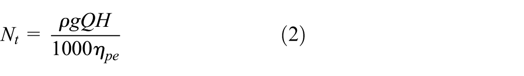
Here, N_t refers to the input power of the pump unit on the tth day (kW); $ρ$ is the density of crude oil (kg/m³); g is the gravity acceleration (m/s²); η_pe is the efficiency of pump unit; H is the total pressure drop (equal to the meter total head) from the entrance inlet to the exit on the tth day; e_d is the price of power (yuan/(t km)); L_R is the interval between the heating station, which, in this article, refers to the length of submarine pipes (m); G_d is the mass flow (t/d); $l_{i}$ is the length of the ith section (m); $ν_{pji}$ is the average viscosity of the ith section (m²/s); $β$ is the relative constant in the flow state; n is the number of tube segments; d is the actual diameter of the waxy pipe after running t days (m); $d_{0}$ is the internal diameter of the pipe when it is not waxy (m); and $δ$ is the wax thickness after running t days (m).

The wax thickness $δ$ can be computed with the wax deposition rate model. In the study of the wax deposition kinetics model, Burger et al.,¹⁵ Hamouda and Ravnoy,¹⁶ Q Huang et al.,¹⁷ Hernandez Perez,¹⁸ and others proposed their own wax deposition models based on Fick’s diffusion law. Among them, the wax deposition model proposed by Q Huang of China University of Petroleum (Beijing) has been successfully applied to the forecast of wax deposition in several long-distance crude oil pipelines in China, including the Wushanlan Pipeline, Adu Pipeline, Zhongyin Pipeline, and Renjing Pipeline. In this article, the wax deposition rate is calculated using the Q Huang model. The specific model is shown in equation (19), and the wax thickness δ is obtained based on the actual parameters of the pipeline:

2. The thermal costs

S_{R} = \frac{c_{y} (T_{1} - T_{2}) e_{y}}{L_{R} η_{R} B_{H}}

(7)

In this formula, S_R is the thermal cost on the tth day (yuan/(t km)), c_y is the heat absorption capacity of crude oil $(kJ / (kg \circ C))$ , T₁ is the outstation temperature on the tth day $(\circ C)$ (the inlet temperature of pipe in this article), T₂ is the in-station temperature on the tth day $(\circ C)$ (the outlet temperature of pipe in this article), e_y is the price of fuel oil (yuan/t), B_H is the calorific value of fuel oil (kJ/kg), and η_R is the efficiency of the heating furnace. The oil temperature along the pipe can be worked out using the Sukhov formula

T_{2} = T_{0} + (T_{1} - T_{0}) e^{- a L_{R}}

(8)

a = \frac{K π d}{G c_{y}}

(9)

The overall coefficient of heat transfer of a waxy pipe should be

K_{W} = \frac{1}{\frac{1}{K} + \frac{δ}{λ'_{ω}}}

(10)

In this formula, K is the overall coefficient of heat transfer of the non-waxed pipe $(W / (m^{2} \circ C))$ , K_W is the overall coefficient of the heat transfer of waxy pipe $(W / (m^{2} \circ C))$ , and $λ'_{ω}$ is the thermal conductivity of the wax deposition layer $(W / (m^{2} \circ C))$ .

3. Unit pigging costs

S_{C} = \frac{e_{c}}{G_{d} Z L_{R}}

(11)

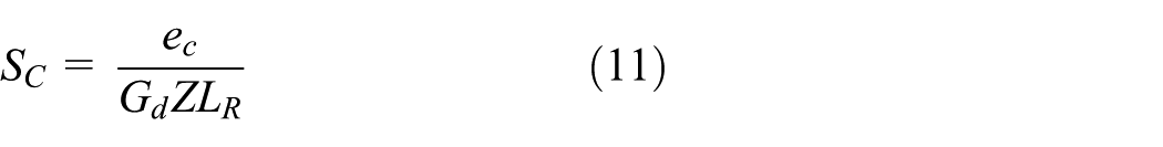
In the formula, e_c is the cost of the single cleaning (yuan).

Constraint conditions

The reduction in the delivery capacity of the pipeline can be calculated using the following formula:

Before waxing

\frac{P_{1}}{ρ g} = \sum_{i = 1}^{n} β \frac{{Q_{1}}^{2 - m} {ν_{pji}}^{m}}{{d_{0}}^{5 - m}} l_{i} + \frac{P_{2}}{ρ g} + Δ Z

(12)

After waxing

\frac{P_{1}}{ρ g} = \sum_{i = 1}^{n} β \frac{{Q_{2}}^{2 - m} ν_{pji}^{m}}{{(d_{0} - 2 δ)}^{5 - m}} l_{i} + \frac{P_{2}}{ρ g} + Δ Z

(13)

Δ Q = Q_{1} - Q_{2}

(14)

In the formula, $P_{1}$ is the inlet pressure of pipe (Pa), $P_{2}$ is the outlet pressure of pipe (Pa), $Δ Z$ is the Z-difference (m), $Δ Q$ is the reduction in the delivery capacity of the pipeline $(m^{3} / s)$ , $Q_{1}$ is the throughput of the non-waxed pipeline (m³/s), and $Q_{2}$ is the throughput of the non-waxed pipeline (m³/s).

2. Hydraulic condition.

Industry standard SY/T 5536-2016 for the operation of crude oil pipeline stipulates that the maximum operation pressure of each point of the running pipeline should not exceed the maximum design pressure. For the transfer stations with different pressure levels, the maximum outbound and inbound pressures of the pipeline should be determined. There is no intermediate station along submarine pipelines, and the outlet pressure of pipelines is usually fixed, and therefore, inlet pressure should satisfy

P_{1} \leq P_{0}

(15)

Here, $P_{1}$ can be worked out using formulas (13) and (14), and $P_{0}$ is the maximum operating pressure.

3. Thermal condition.

Theoretically, when the inlet temperature is fixed, the process of heating from the pipeline medium to the soil environment, that is, the forced convection from the oil stream to the pipe wall, involves three steps: the heat conduction of the steel tube wall, the asphalt insulating layer or the insulation layer, and natural convection from ectooecium of the pipe to the soil environment. A waxy layer will form on the inner wall after a period of operation, which means that the insulating layer will be strengthened and heat resistance will grow. Consequently, the total heat transfer coefficient decreases.⁸ Compared to the non-waxed pipe, the outlet temperature of the waxy pipe will be higher than its counterpart. It can be concluded that on the condition of thermal constraints, the outlet temperature should be set at a higher level than the solidifying point of crude oil. That is to say, $T_{2} < T_{Freezing point}$ (T₂ refers to the outlet temperature before pipe waxing $(\circ C)$ ). The pipeline operation specification generally requires that the pipeline outlet temperature be at least 3°C–5°C higher than the freezing point.¹⁹

Before the pipe waxes, numerous sections will be divided, each of whose length shall be assumed as dx, and the thermal balance relationship of each section should be²⁰

K π d_{0} (T - T_{0}) dx = - G c_{y} dT - κ G \frac{\partial ε_{y}}{\partial T} dT

(16)

In this formula, $d_{0}$ is the internal diameter of the pipeline (m), G is the mass flow (kg/s), c_y is the heat absorption capacity of crude oil (J/(kg °C)), $κ$ is the crystalline latent heat of wax (J/kg), $\partial ε_{y} / \partial T$ is the proportion of wax when the temperature declines by $1 \circ C$ accounting for the quality of crude oil, and $T_{0}$ is the ambient temperature of the buried depth of the pipe $(\circ C)$ . Integrating equation (16), we can get the following result

T_{2} = T_{0} + (T_{1} - T_{0}) \exp (- \frac{K π d_{0} L_{R}}{G c_{y} + κ G \frac{\partial ε_{y}}{\partial T}})

(17)

In this equation, $T_{1}$ is the inlet temperature of the pipeline $(\circ C)$ , and $T_{2}$ is the outlet temperature of the pipeline $(\circ C)$ . When the pipe embraces certain wax thickness

T_{2} = T_{0} + (T_{1} - T_{0}) \exp (- \frac{K_{w} π d L_{R}}{G c_{y} + κ G \frac{\partial ε_{y}}{\partial T}})

(18)

The solution of the model

To take safe operation of the pipeline into consideration, when its throughput declines by 3%, the corresponding cleaning time represents the maximum cycle. However, wax thickness somewhat affects the total cost; different thicknesses correspond to different economic pigging cycles, and therefore, the optimal cycle t_max with a different thickness should be determined before we solve the model. According to the figure t_max, this will yield a different cycle. The steps to solve the model are as follows:

Step 1. Fix different wax thicknesses and calculate the maximum pigging cycle t_max.

Step 2. Find an economic pigging cycle among those maximum figures. The detailed calculation is shown in Figure 2.

Figure 2.

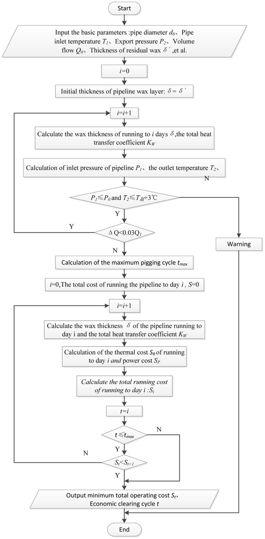
Block diagram of the calculation of the economic pigging cycle with different wax thicknesses.

Examples analysis

Overview of the outbound pipeline from the central processing platform to the terrestrial terminal in the M Oilfield Group

The output of crude oil in the M Oilfield Group has been rapidly decreasing in the recent years. As a result, the throughput of outbound pipeline is 50% lower than projected. These pipelines have been deteriorating and transporting low volumes. If the volumes are so small that pipelines will work unstably, and the operation pressure will continuously increase while throughput decreases constantly, the entire line may stop functioning. Even worse, wax content of crude oil in this field accounts for 23.142%. Wax deposition will reduce the flow area of the pipe. If the pipe is not cleaned for a long time, serious wax deposition will occur in the pipe at a local position, resulting in the plugging of the pig during pigging. Therefore, it is necessary to determine a reasonable and reliable economic clean-up cycle for the pipeline.

The external pipeline from the central processing platform of the M Oilfield Group to the land terminal is composed of two parts, namely, a subsea buried pipeline and a land-suspended pipeline. The basic parameters of the pipeline are shown in Table 1.

Table 1.

Basic parameters of the pipelines from the center processing platform to the onshore terminal of the M Oilfield Group.

	The sea tube	The land tube
Inner diameter	16″ (406.4 mm O.D. × 14.3 mm W.T.)	16″ (406.4 mm O.D. × 11.1 mm W.T.)
Outer diameter	22″ (559 mm O.D. × 15.9 mm W.T.)	None
The length of the pipe	44.2 km	14.6 km
Roughness	0.04572 mm	0.04572 mm
Total heat transfer coefficient	0.85 W/(m² K)	0.9 W/(m² K)

Prediction of wax deposition characteristics in the M Oilfield Group Center treatment platform to overland terminal pipeline

To calculate the economic pigging cycle, the first step we should take is to figure out the law of the wax deposition in the pipeline.²¹ In this article, the Q Huang et al.’s¹⁷ pervasive wax model is used to calculate the thickness of wax. According to the actual operating parameters of the external pipeline from the M Oilfield Group Center treatment platform to the land terminal, the wax deposition model should be computed using this formula

W = 992.3 τ_{ω}^{- 0.5532} \frac{1}{μ} \frac{dC}{dT} {(\frac{dT}{dr})}^{0.7618}

(19)

Based on this model, the MATLAB software is used to formulate the program to calculate the waxing of the pipeline from the M Oilfield Group Center treatment platform to the land terminal. When the flow rate is 146.37 m³/h, wax deposition conditions at different inlet temperatures are shown in Figure 3, and the corresponding outlet temperature is shown in Figure 4. This lays the foundation for calculating the pigging cycle.

Figure 3.

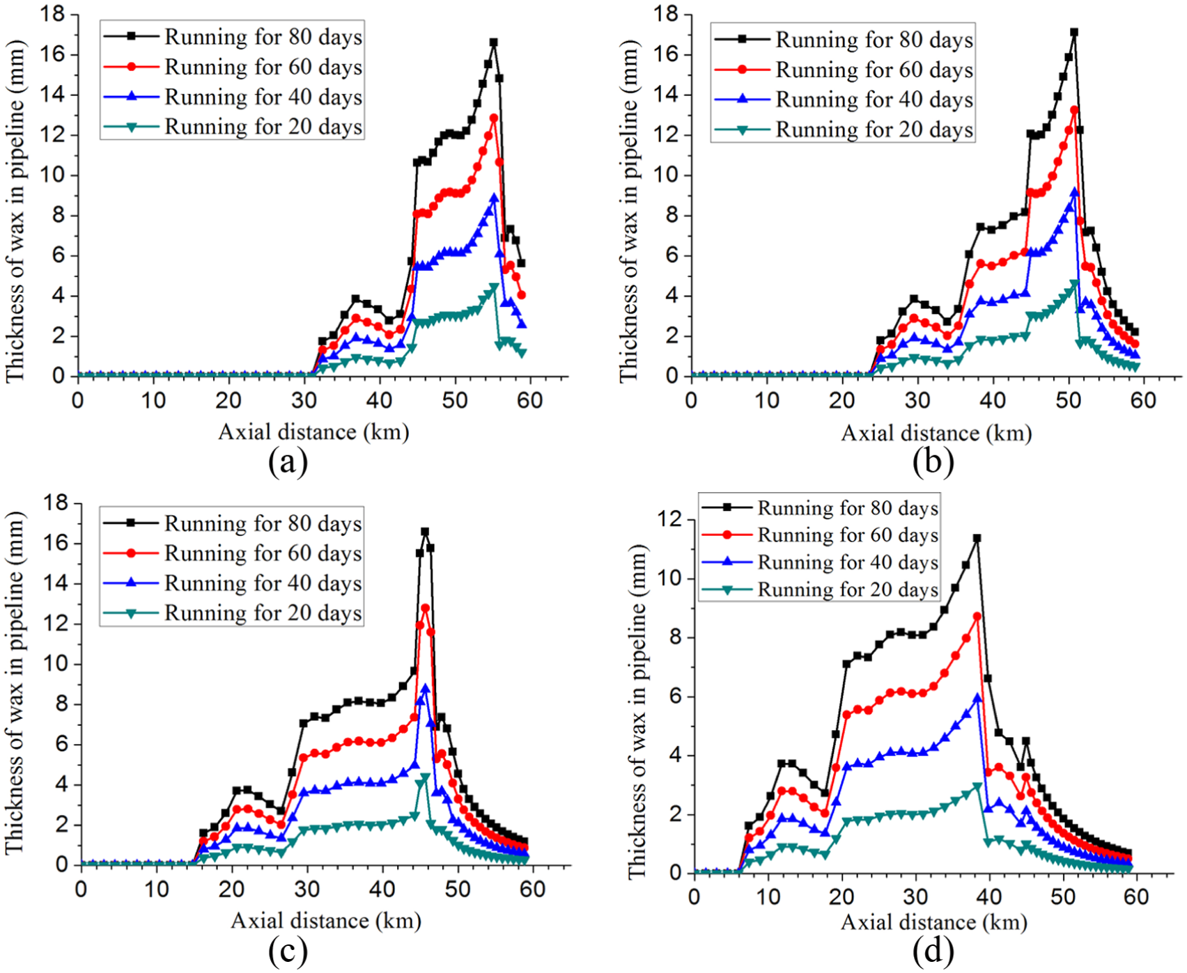
When the transportation amount is 146.37 m³/h, the variation in wax deposition thickness along the pipeline with different inlet temperatures: (a) thickness of the paraffin wax at the inlet temperature of 70°C, (b) thickness of the paraffin wax at the inlet temperature of 65°C, (c) thickness of the paraffin wax at the inlet temperature of 60°C, and (d) thickness of the paraffin wax at the inlet temperature of 55°C.

Figure 4.

At different inlet temperatures, the outlet temperature changes with the running time.

Influence of the pipeline inlet temperature on the economic pigging cycle

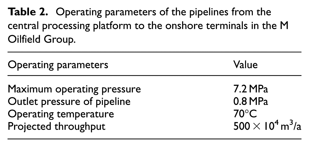
To calculate the economic pigging cycle of pipelines under different operating conditions, the first step we need to take is to figure out the operating costs and other parameters of the pipeline (Tables 2 and 3). The operating costs and parameters of the pipelines from the center processing platform to the onshore terminal of the M Oilfield Group are shown in Table 2.

Table 2.

Operating parameters of the pipelines from the central processing platform to the onshore terminals in the M Oilfield Group.

Operating parameters	Value
Maximum operating pressure	7.2 MPa
Outlet pressure of pipeline	0.8 MPa
Operating temperature	70°C
Projected throughput	500 × 10⁴ m³/a

Table 3.

The operating parameters of the pipeline of the M Oilfield Group Center.

Operating parameters	Value
Fuel oil calorific value (J/kg)	4.2 × 10⁷
Fuel oil price (yuan/t)	3500
Electricity price (yuan/(kW h))	0.9
Reheating furnace efficiency	0.9
Efficiency of pump unit	0.85
Cost of disposable cleaning (yuan)	8000

The electricity price of 0.9 yuan/(kW h) is equivalent to approximately US$139.6 (US$/MW h).

An observation of the operation reveals that the maximum operating pressure is 7.2 MPa, the outlet pressure of the pipeline is 0.8 MPa, and the operating temperature is 70°C. This article will pick up 70°C, 65°C, 60°C, and 55°C for individual analysis. According to the data in Table 3, the effect of the inlet temperature on the pigging cycle will be analyzed. When the flow rate is 146.37 m³/h, the average wax thickness of the pipeline is shown in Figure 5.

Figure 5.

The average wax thickness of pipeline with different inlet temperatures.

From Figure 5, it is clear that, with time, the average wax thickness of the pipeline increases linearly. When the flow stays stable, the higher the inlet temperature of the pipeline is, the lower the average wax thickness is. After calculation, we can see that when the pipeline transport capacity reduces by 3%, the average thicknesses of the wax corresponding to different inlet temperatures of 70°C, 65°C, 60°C, and 55°C are 1.49, 1.54, 1.58, and 1.62 mm, respectively. The corresponding economic pigging cycle is shown in Figure 6.

Figure 6.

The economic pigging cycle with different inlet temperatures.

From Figure 6, we can see that as the pipeline keeps working, the total costs of pipeline operations continue to decrease. When the volume is fixed, the higher the inlet temperature is, the higher the total costs of the pipeline are, which results from the increase in the thermal costs. It can be concluded in Figure 3 that, as it has operated for 40 days, the thickness of the local wax has reached 10 mm, and throughput efficiency has declined to 3%. However, there exists no theoretical minimum cost, because of low waxy efficiency. When the inlet temperatures are 70°C, 65°C, 60°C, and 55°C, the corresponding pigging cycles are 33, 32, 31, and 30 days.

The effect of throughput on the period of economic pigging

When the inlet temperature is 70°C, the average wax thickness of pipelines with different transportation amounts is shown in Figure 7 and the economic pigging cycles with different transportation amounts is shown in Figure 8.

Figure 7.

The average wax thickness of pipeline with different transportation amounts.

Figure 8.

The economic pigging cycle with different transportation amounts.

As shown in Figure 7, as days pass, the average wax thickness in the pipeline increases linearly. When the inlet temperature is fixed, the greater the volume is, the lower the average wax thickness is. We can calculate that when throughput is reduced by 3%, the average thicknesses of the wax corresponding to 146.37, 138.24, 130.11, and 121.98 m³/h for different transmission volumes are 1.49, 1.45, 1.40, and 1.34 mm. The pigging cycles are shown in Figure 8.

As shown in Figure 8, we can see that as days pass, the total costs of pipeline operations are decreasing. The reason is that the wax thickness becomes larger and the total heat transfer coefficient of the pipe decreases. As a result, the thermal costs decline. When the inlet temperature stays at 70°C, the corresponding pigging cycles of 146.37, 138.24, 130.11, and 121.98 m³/h are, respectively, 33, 31, 29, and 27 days.

The influence of the thickness of residual wax on the period of economic pigging

Figures 9 and 10 show, respectively, the total operating costs and the economic pigging cycle for different thicknesses of residual wax at different inlet temperatures of the pipeline when throughput is maintained at 146.37 m³/h. It is shown in Figure 9 that when throughput remains fixed, operation costs will increase as the inlet temperature increases because growing thermal costs will increase the total cost. When the remnant wax thickness is 0.4 mm, the total costs of the pipeline are the lowest. Therefore, while pigging, wax thickness should be maintained at 0.4 mm. At the same time, it can be concluded from Figure 10 that, with an increase in the wax thickness, the gap between pigging cycles at different inlet temperatures grows. The reason is that wax plays a role in heating the pipeline, which is helpful in postponing the temperature of the oil flow, in slowing down the wax deposition rates, and in reducing the delivery efficiency.

Figure 9.

The total operating costs with different inlet temperatures and different remnant wax thicknesses.

Figure 10.

The economic pigging cycle with different inlet temperatures and different remnant wax thicknesses.

Figures 11 and 12 show, respectively, the total operating cost and the pigging cycle for different thicknesses of residual wax at different transportation amounts when the inlet temperature is 70°C. As shown in Figure 11, when the inlet temperature is fixed, the larger the throughput is, the less the total cost is. When throughput increases, the total capacity grows, too. However, on the condition of stable inlet oil temperature and environmental temperature, the loss of thermality along the pipeline is constant—that is to say, the proportion of thermal loss is reduced. In addition, as throughput increases, friction increases and plays a role in heating pipelines; consequently, thermal costs reduce. When remnant wax thickness is maintained at 0.2–0.4 mm, the total cost is the lowest. From Figure 12, as wax thickness increases, the gap between cycles will grow.

Figure 11.

The total operating cost with different transportation amounts and different remnant wax thicknesses.

Figure 12.

The economic pigging cycle with different transportation amounts and different remnant wax thicknesses.

Overall, a 3%-drop in delivery capacity can be a safety limit when calculating a pigging cycle. The result conforms to results from previous experiences and makes the cost the lowest. If we calculate the economic pigging cycle according to the general method, it can be seen from Figure 1 that the pigging period is close to 1000 days. Combined with the analysis of Figure 3, the local wax deposit thickness of the pipeline has caused serious hidden trouble, or even a blockage, to the actual pipeline operation.

Conclusion

The economic pigging model established in this article can almost accurately predict an economic cycle when sea pipelines work at a low volume. Theoretically, the lowest cost exists. However, since each pipeline works differently, the lowest cost may not appear until it has been in operation for a long time and/or when delivery capacity has exceeded the security limit. Therefore, when establishing the economic cycle, it is necessary to take both delivery capacity and economy into consideration.

When throughput is fixed, the lower the inlet temperature and total costs are, the shorter the relevant cycle is. When the inlet temperature stays stable, the throughput is larger, the total costs are at the lowest, and the cycle is longer. Wax thickness has a certain effect on operation costs. Keeping a reasonable thickness helps cut down total costs.

The gelation mechanism increases and then decreases with decreasing bulk fluid temperature, which will have a certain effect on the wax deposition process. However, these effects are missing in this article. Future research should include the gelation process.

Footnotes

Handling Editor: Roslinda Nazar

Declaration of conflicting interests

The author(s) declared no potential conflicts of interest with respect to the research, authorship, and/or publication of this article.

Funding

The author(s) disclosed receipt of the following financial support for the research, authorship, and/or publication of this article: This work was supported by the Sichuan Provincial Key Discipline Construction Foundation of China (No. SZD0426).

ORCID iD

Diwen Chen

References

Wang

Liu

Statistics and analysis of subsea pipeline accidents of CNOOC. China Offshore Oil Gas 2017; 29: 157–160.

Zhenxing

Analysis on operation characteristics of waxy crude pipeline with low throughput and research on safety protection technology. Daqing, China: Northeast Petroleum University, 2016.

Chala

Sulaiman

Japper-Jaafar

et al . Effects of cooling regime on the formation of voids in statically cooled waxy crude oil. Int J Multiphas Flow 2015; 77: 187–195.

Ronningsen

HP.

Production of waxy oils on the Norwegian continental shelf: experiences, challenges, and practices. Energ Fuel 2012; 26: 4124–4136.

Chala

Sulaiman

Japper-Jaafar

Flow start-up and transportation of waxy crude oil in pipelines—a review. J Non-Newton Fluid 2018; 251: 69–87.

Sulaiman

Biga

Chala

GT.

Injection of non-reacting gas into production pipelines to ease restart pumping of waxy crude oil. J Petrol Sci Eng 2017; 152: 549–554.

Jiping

Xinyi

Baojian

et al . Calculation of the thickness of wax and investigation on the optimization pigging period of buried hot waxy crude pipeline. Contemp Chem Ind 2016; 45: 545–548.

Liu

Wang

Cheng

et al . The study of pipe-line wax deposition law and pigging period for Daqing waxy crude oil. Acta Pet Sin 2012; 33: 892–897.

Yue

Wen

Effect of wax deposition on energy consumption in hot wax crude pipeline with low through-put. J Fushun Pet Inst 2002; 22: 38–40.

10.

Jiang

G-Y

Zhang

W-X

Zhou

S-D

et al . Pigging period study for oil pipeline with low through-put. J Fushun Pet Inst 2003; 23: 46–49.

11.

Zhou

Wang

Zhao

Investigation on the optimization pigging period of buried hot waxy crude pipeline. Oil Gas Storage Transp 2006; 25: 15–17.

12.

Ding

Cai

Wang

et al . Differences in pigging standards between China and Russia. Oil Gas Storage Transp 2013; 32: 1018–1021.

13.

Cheng

Yan

Jinzhou

SY/T 5536-2016 specification for operation of crude oil pipelines. Beijing, China: Petroleum Industry Press, 2016.

14.

Huazhuo

Lei

et al . Summary of pigging technology for long-distance pipeline at home and abroad. Total Corros Control 2017; 31: 6–10.

15.

Burger

Perkin

Striegler

JH.

Studies of wax deposition in the trans Alaska pipeline. J Petrol Technol 1981; 33: 1075–1086.

16.

Hamouda

Ravnoy

. Prediction of wax deposition in pipelines and field experience on the influence of wax on drag-reducer performance. In: The 24th annual offshore technology conference, Houston, TX, 4–7 May 1992, pp. 669–679. Houston, TX: Offshore Technology Conference.

17.

Huang

Zhang

Unified wax deposition model. Acta Pet Sin 2008; 29: 459–462.

18.

Hernandez Perez

. Investigation of single-phase paraffin deposition characteristics. Tulsa, OK: The University of Tulsa, 2002.

19.

Yang

Pipeline design and management. Donying, China: China University of Petroleum Press, 2013.

20.

Dafan

Pipeline design and management. Beijing, China: Petroleum Technology Press, 1986.

21.

Qiyu

Qing

Xindong

et al . The influence of uneven wax distribution along the pipeline on the calculation of the thickness of the wax layer. Oil Gas Storage Transp 2008; 27: 24–26.

Economic pigging cycles for low-throughput pipelines

Abstract

Keywords

Introduction

Mathematical modeling and techniques

The establishment of a pigging model

Constraint conditions

The solution of the model

Examples analysis

Overview of the outbound pipeline from the central processing platform to the terrestrial terminal in the M Oilfield Group

Prediction of wax deposition characteristics in the M Oilfield Group Center treatment platform to overland terminal pipeline

Influence of the pipeline inlet temperature on the economic pigging cycle

The effect of throughput on the period of economic pigging

The influence of the thickness of residual wax on the period of economic pigging

Conclusion

Footnotes

Declaration of conflicting interests

Funding

ORCID iD

References