Thermal characteristic analysis of Z-axis guideway based on thermal contact resistance

Abstract

The Z-axis feeding system of large computer numerical control (CNC) gear grinding machine tools generates lots of heat during processing, which leads to tilt and pitch deformation of the Z-axis guideway and reduces the machining accuracy. In view of this situation, a three-dimensional finite element analysis method is proposed to conduct transient thermal-structural coupling analysis of the Z-axis guideway and feeding system. Considering the microscopic contact state on machine tool joint surfaces and using the root mean square measurement method, the fractal parameter is identified and the thermal contact resistance at the joints is calculated. The friction heat on the guideway is calculated and the thermal value of the motor is obtained. Then, the heat generation rate of the bearing and the screw nut is calculated according to the friction torque. The convective heat transfer coefficient is determined according to the Reynolds number and the Nusselt number. The finite element model is established to obtain the finite element simulation results of thermal error. Finally, the experimental platform for measuring the temperature and thermal deformation of the large computer numerical control gear grinding machine tool is set up, and the accuracy and reliability of the method is verified.

Introduction

Large computer numerical control (CNC) gear grinding machine tool is mainly used to process large and high-precision gears in the fields of aviation, ships, wind power, engineering machinery, and so on. ¹ The machine tools will generate a lot of heat due to working for a long time; because the gears with large size work for a long time, the machine tools generate a lot of heat and result in the thermal deformation of lathe bed, column, guideway, spindle, and other major components. Therefore, there is a strong correlation between the workpiece error and the thermal deformation of the machine tools. With an increase in cutting speed and cutting power, the error caused by thermal deformation accounts for about 70% of the total error of machine tools. ² In order to reveal the laws of this thermal deformation of large CNC gear grinding machine tools and improve machining accuracy, it is necessary to conduct research on the thermal error of large CNC gear grinding machine tools.

In recent years, more and more scholars have devoted themselves to the thermal analysis of machine tools and have made great progress. Xu et al. ³ built the coupling mechanism of the machine tool feeding system model based on mechanical and thermal characteristics. Holkup et al. ⁴ proposed a transient analysis method for the spindle thermal-structural model, calculated the temperature distribution and thermal deformation of the spindle thermal model, and updated the thermal-structural model according to the thermal deformation. Zhao et al. ⁵ analyzed the temperature distribution and thermal deformation of the spindle with the finite element method (FEM), and the thermal error model was established. Chen et al. ⁶ proposed a thermal-structural error model of a spindle for high-precision machine tools and predicted the variation of motion error caused by thermal effect on a machine worktable during processing. Bossmanns and Tu ⁷ presented a finite difference method (FDM) to characterize the power distribution and thermal error of a high-speed spindle, including the characterization of heat transfer and heat dissipation. Su et al. ⁸ built an integrated thermo-hydro-mechanical coupling model of the hydrostatic spindle system, considering the interaction of the temperature field, thermal deformation, and oil film thickness based on the finite volume element method (FVEM). Wang et al. ¹ proposed a thermal deformation theory model for a large CNC gear grinding machine tool based on the thermal expansion theory of metal materials, which can further improve machining precision.

In the above models, the heat source and heat transfer as the main boundary conditions for thermal error analysis were taken into account. However, due to the rough surface morphology, contact area, and interfacial pressure on the surfaces of the machine tool joint, the thermal contact resistance (TCR) exists in the heat transfer process, which results in the inaccuracy of simulation results and cannot be ignored because of the discontinuity and the strong nonlinear relationship during the heat transfer process. Liu et al. ⁹ built the TCR network model for the spindle bearing block of precision horizontal machining center and analyzed the steady-state thermal and transient thermal model in consideration of the deformation affected by TCR. Ma et al. ¹⁰ presented a TCR model based on fractal contact mechanics analysis by measuring the surface morphology parameters and identifying the fractal parameters. Su et al. ¹¹ proposed a finite element fractal method by an integrated fractal theory and FEM; this method analyzed the thermal characteristics of an ultra-precision machine tool under the influence of TCR.

The framework of this article is arranged as follows. Section “TCR fractal model” introduces the Z-axis feeding system of the large CNC gear grinding machine tool, and a fractal contact model is proposed based on the Weierstrass–Mandelbrot (W-M) function and the root mean square measurement (RMSM) method. The TCR model is established by integrating the Hertz theory and the fractal theory. In section “Analysis of the simulation for thermal error,” the calculation method of boundary conditions is discussed. The friction heat on the guideway, thermal power of the motor, and heat generation rate of the bearing and screw nut are calculated. According to the Reynolds number and the Nusselt number, the convection heat transfer coefficient of machine tool parts is determined. The thermal error model of the Z-axis feeding system is established based on the above boundary conditions and the TCR. In section “Experiment,” the thermal error measurement experiments are carried out to verify the validity of the model and the experimental data are analyzed. Section “Conclusion” presents the conclusion of the previous analysis.

TCR fractal model

Z-axis feeding system of large CNC gear grinding machine tools

In this article, the object of the study is the Z-axis guideway and feeding system of large CNC gear grinding machine tools, as shown in Figure 1. The main components of the Z-axis feeding system are motor, coupling, lead screw, screw nut, guideway, column, carriage, and other components. Because of the high feeding rate and cutting speed during the gear machining process, to ensure the stability of the process, the weight of the Z-axis carriage has greatly increased when designing large CNC gear grinding machine tools. The total mass is up to 6000 kg. In addition, during the lengthy grinding process, the carriage and the guideway carry on relative motion continuously, which will produce a large amount of friction heat. Coupled with the impact of the heating of the motor, cutting heat, and other heat sources, the temperature of the column and the guideway gradually increases, which in turn produces a corresponding thermal deformation and causes guideway tilt, deflection, pitching, and linear positioning error. Thermal deformation results in a relative position error between the grinding wheel and the gear workpiece production, which affects the processing precision of the gear seriously.

Figure 1.

The structure diagram of a large CNC gear grinding machine tool.

Fractal contact model

W-M fractal function

Metal surface morphology is an important factor that affects the surface quality of machined surfaces and the surface matching of friction pairs. Rough surface profile curve is an important method to characterize surface topography. The machined surface contour curve can be described by fractal theory owing to its self-similarity. The fractal theory can be used to characterize the machined surface and fully reflect the details of the surface contour without depending on the accuracy of the measuring equipment. As shown in Figure 2, the W-M fractal curve is the same as the surface contour curve approximately. Namely, the surface contour curve and the W-M fractal curve are all continuous, non-derivable, and self-similar.

Figure 2.

(a) The surface contour curve and (b) the W-M fractal curve.

Therefore, the W-M fractal curve is used to describe the features of the machined surface contour curve; the expression of the W-M fractal curves function is ¹²

$$z(x)=G^{(D-1)}\sum _{n=n_l}^{\infty }{\gamma }^{-(2-D)n}\cos (2\pi {\gamma }^{n}x),1<D<2,\gamma >1$$

(1)

where D is the fractal dimension of the surface profile; G is the characteristic length scale of the surface; x is the horizontal coordinates of the contour; γ is a constant greater than 1, where γ = 1.5 is a suitable value for high spectral density and for phase randomization; n is the spatial frequency ordinal number; γⁿ is the spatial frequency of the contour curve, equal to the reciprocal of the sampling length Lⁿ of the rough surface (γⁿ = 1/Lⁿ ); and n_l is the ordinal number corresponding to the lowest cut-off frequency of the contour curve.

Fractal parameter identification

The method of RMSM has a better effect on the characterization of machined surface profiles. So the method of RMSM is used to identify the fractal parameters of surface morphology on the machine tool joint surface. The RMSM method regards the surface contour curve as a space sequence Z(τ); the space sequence Z(τ) with fractal property satisfies the following scaling relation ¹³

$$Z(\tau )-Z\left({\tau }_0\right)=\zeta {|\tau -{\tau }_0|}^{2-D}$$

(2)

If τ₀ = 0, Z(0) = 0, then the variance or covariance of time series is

$$\mathrm{Var}(\tau )=E\left\{{[Z\left(\tau \right)-\overline{Z\left(\tau \right)}]}^2\right\}~{\tau }^{4-2D}$$

(3)

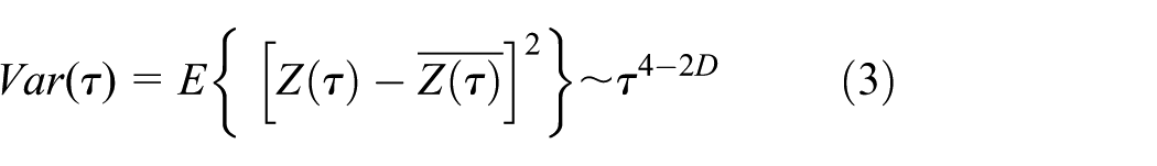
or

$$\sigma (\tau )={\left[\mathrm{Var}\left(\tau \right)\right]}^{\frac{1}{2}}=G·{\tau }^{2-D}$$

(4)

where σ(τ) is the RMSM; it represents the average value or the mean square root of the variance; τ is the scale, which is the arbitrary value of the data interval; equation (4) expresses the RMSM and the space interval scaling of the space sequence; it shows that the square mean difference and regional scale τ are power exponential relations in area τ and the power exponent associated with fractal dimension. View a digitized surface profile as a spatial sequence, using n scales τ_i (i = 1, 2, …, n) to calculate its mean square σ(τ). σ(τ) = G^τ2-D is the logarithm taken on both sides, and then we obtain the following relationship curve

$$\log \sigma (\tau )=(2-D)\log \tau +\log G$$

(5)

Through linear fitting, we can obtain a straight line using equation (5), the fractal dimension D can be obtained from the slope of the line α, and the characteristic length scale G can be obtained from the intercept of line A

$$D=2-\alpha$$

(6)

$$\log G=A$$

(7)

Area distribution of asperities

Mandelbrot found that the number N (micro-contact area A exceeded a certain value a) and a obeyed the following relations ¹²

$$N(A>a)=k{a}^{-D/2}$$

(8)

where k is the scaling factor.

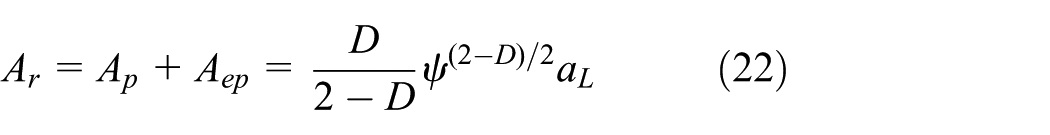
The area distribution function of asperities can be obtained by fractal theory

$$n(a)=\frac{D}{2}{\psi }^{(2-D)/2}{a_L}^{D/2}{a}^{-(D+2)/2}$$

(9)

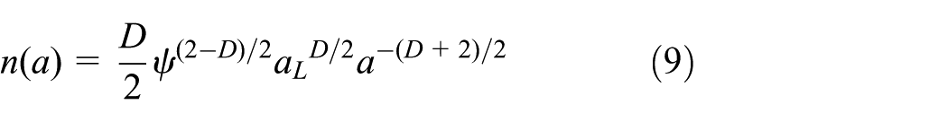
where a_L is the maximum truncated area of the asperities, a is the actual contact area of the asperities, and Ψ is the expanding factor of the fractal region. The solution of Ψ can be solved by the transcendental equation as follows

$$\frac{{\psi }^{(2-D)/2}-{(1+{\psi }^{-D/2})}^{-(2-D)/2}}{(2-D)/D}=1$$

(10)

Fractal topography of a single asperity

In fractal theory, the contact between two rough surfaces can be identified as the contact between a rigid plane and a rough surface, as shown in Figure 3. Before the deformation, the asperity profile is a cosine wave function

$$z(x)=G^{(D-1)}l{\prime }^{(2-D)}\cos \left(\frac{\pi x}{l\prime }\right);-\frac{l\prime }{2}<x<\frac{l\prime }{2}$$

(11)

Figure 3.

The deformation of a single asperity.

Figure 3 illustrates an asperity truncated by a rigid plane and the deformation of a single asperity.

Deformation at the top of asperity δ can be expressed as follows

$$\delta =z(0)=G^{(D-1)}l{\prime }^{(2-D)}=2^{(2-D)}{G}^{(D-1)}{\left(\frac{a\prime }{\pi }\right)}^{(2-D)/2}$$

(12)

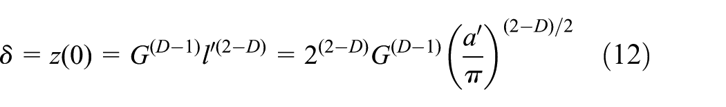
where a is the actual contact area of the asperity, a′ is the truncated area of the asperity, l′ is the truncated diameter of the asperity, and l is the actual contact diameter.

According to Hertz theory, the elastic load of asperity is ¹⁴

$$P=\frac{4}{3}E{R}^{\frac{1}{2}}{\delta }^{\frac{3}{2}}$$

(13)

where E is the equivalent elastic modulus, and $E=(((1-v_1^2)/E_1)+((1-v_2^2)/E_2)){)}^{-1}$ , where E₁, E₂, v₁, v₂ represent Young’s elastic modulus and Poisson’s ratio of the two contacting materials, respectively. R is the true curvature radius of circular contour at the top of the asperity, R =2^Da′^D/2/π^(4+D)/2G^–1.

When elastic deformation occurs in the asperity, the relationship between the actual area a and the truncated area a′ before deformation is a = a′/2.

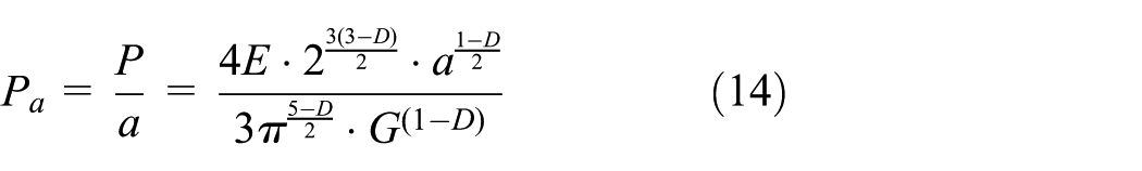
Plugging equations (10) and (12) into equation (13), the average contact pressure on the asperity can be expressed as follows

$$P_a=\frac{P}{a}=\frac{4E·2^{\frac{3(3-D)}{2}}·a^{\frac{1-D}{2}}}{3{\pi }^{\frac{5-D}{2}}·G^{(1-D)}}$$

(14)

According to Hertz theory, the maximum deformation of the asperity can be expressed as follows

$$\delta ={\left(\frac{3\pi p_0}{4E}\right)}^{2}R$$

(15)

where p₀ is the average pressure, and the maximum pressure is 1.5 times the average pressure. ¹⁵

The initial pressure of the elastic deformation of the asperity is p_c = Kσ_y, where K is a factor that is associated with hardness H and yield strength σ_y (K = σ_y/H).

Plugging p_c into equation (15), the critical deformation δ_ec of elastic deformation of asperity can be expressed as follows

$${\delta }_{\mathrm{ec}}={\left(\frac{3\pi K{\sigma }_y}{4E}\right)}^2·R$$

(16)

When the deformation δ of the asperity satisfies the condition δ < δ_ec, elastic deformation occurs on the contacting asperities.

When a = a_ec, δ = δ_ec, elastic deformation begins to occur, and the contact area of the asperity is

$$a_{\mathrm{ec}}=\frac{G^2}{8}{\left(\frac{3K{\sigma }_y}{E{\pi }^{(D+1)/2}}\right)}^{\frac{2}{1-D}}$$

(17)

When the deformation δ of the asperity satisfies the condition δ < δ_ec, elastic deformation occurs on the contacting asperities. Therefore, the elastic deformation condition of the asperity can be expressed by contact area a > a_ec.

Critical plastic deformation contact area

According to Johnson’s ¹⁶ theory, when El′/σ_yR ≈ 60, complete plastic deformation occurs in the contact asperity. When complete plastic deformation occurs, the relationship between the actual micro-contact area a and the truncated area of the asperity a′ obeys the following relationship: a = a′.

The critical plastic deformation contact area of the asperity is

$$a_{\mathrm{pc}}=\frac{G^2}{4}{\left(\frac{E{\pi }^{\frac{3+D}{2}}}{60{\sigma }_y}\right)}^{\frac{2}{D-1}}$$

(18)

where a_pc is the critical deformation when complete plastic deformation occurs.

When the micro-contact area of the asperity is smaller than the critical plastic deformation micro-contact area a_pc, complete plastic deformation occurs in the asperity; when the micro-contact area of asperity is larger than the critical plastic deformation micro-contact area a_pc and smaller than the critical elastic deformation, elastic–plastic deformation occurs in the asperity.

Total contact area of asperities

According to the analysis of the fractal contact model for a single asperity, the micro-contact state can be divided into three types: complete plastic deformation state, elastoplastic deformation state, and elastic deformation state. By analyzing the micro-contact area, the three contact types show different micro-contact states, as shown in Figure 4.

Figure 4.

The schematic diagram of deformation regimes.

• Total actual contact area of micro-contact

• When a_pc < a_L < a_ec, the micro-contact point is elastic–plastic deformation state, namely, plastic deformation and elastic–plastic deformation occur in asperities. In this state, the complete plastic contact area is

  $$\begin{array}{c}\multicolumn{1}{c}{A_p=\underset{0}{\overset{a_{\mathrm{pc}}}{\int }}a·n(a)\mathrm{da}}\\ =\underset{0}{\overset{a_{\mathrm{pc}}}{\int }}a\frac{D}{2}{\psi }^{(2-D)/2}{a_L}^{D/2}{a}^{-(D+2)/2}\mathrm{da}\hfill \\ =\frac{D}{2-D}{\psi }^{(2-D)/2}{a_L}^{D/2}{a_{\mathrm{pc}}}^{(2-D)/2}\hfill \end{array}$$

  (20)

Elastic–plastic contact area

$$\begin{array}{c}\multicolumn{1}{c}{A_{\mathrm{ep}}=\underset{a_{\mathrm{pc}}}{\overset{a_L}{\int }}a·n(a)\mathrm{da}}\\ =\underset{a_{\mathrm{pc}}}{\overset{a_L}{\int }}a·\frac{D}{2}{\psi }^{(2-D)/2}{a_L}^{D/2}{a}^{-(D+2)/2}\mathrm{da}\hfill \\ =\frac{D}{2-D}{\psi }^{(2-D)/2}[a_L-{a_L}^{D/2}{a_{\mathrm{pc}}}^{(2-D)/2}]\hfill \end{array}$$

(21)

Total contact area

$$A_r=A_p+A_{\mathrm{ep}}=\frac{D}{2-D}{\psi }^{(2-D)/2}{a}_L$$

(22)

• 3. When a_L > a_ec, the micro-contact point is elastic deformation state, namely, plastic deformation, elastic–plastic deformation, and plastic deformation occur in asperities. In this state, the complete plastic contact area is

  $$\begin{array}{c}\multicolumn{1}{c}{A_p=\underset{0}{\overset{a_{\mathrm{pc}}}{\int }}a·n\left(a\right)\mathrm{da}}\\ =\underset{0}{\overset{a_{\mathrm{pc}}}{\int }}a\frac{D}{2}{\psi }^{(2-D)/2}{a_L}^{D/2}{a}^{-(D+2)/2}\mathrm{da}\hfill \\ =\frac{D}{2-D}{\psi }^{(2-D)/2}{a_L}^{D/2}{a_{\mathrm{pc}}}^{(2-D)/2}\hfill \end{array}$$

  (23)

Elastic–plastic contact area

$$\begin{array}{c}\multicolumn{1}{c}{A_{\mathrm{ep}}=\underset{a_{\mathrm{pc}}}{\overset{a_{\mathrm{ec}}}{\int }}a·n\left(a\right)\mathrm{da}}\\ =\underset{a_{\mathrm{pc}}}{\overset{a_{\mathrm{ec}}}{\int }}a·\frac{D}{2}{\psi }^{(2-D)/2}{a_L}^{D/2}{a}^{-(D+2)/2}\mathrm{da}\hfill \\ =\frac{D}{2-D}{\psi }^{(2-D)/2}{a_L}^{D/2}[{a_{\mathrm{ec}}}^{(2-D)/2}-{a_{\mathrm{pc}}}^{(2-D)/2}]\hfill \end{array}$$

(24)

Elastic contact area

$$\begin{array}{c}\multicolumn{1}{c}{A_e=\underset{a_{\mathrm{ec}}}{\overset{a_L}{\int }}a·n\left(a\right)\mathrm{da}}\\ =\underset{a_{\mathrm{ec}}}{\overset{a_L}{\int }}a·\frac{D}{2}{\psi }^{(2-D)/2}{a_L}^{D/2}{a}^{-(D+2)/2}\mathrm{da}\hfill \\ =\frac{D}{2-D}{\psi }^{(2-D)/2}[a_L-{a_L}^{D/2}{a_{\mathrm{ec}}}^{(2-D)/2}]\hfill \end{array}$$

(25)

Total contact area

$$A_r=A_p+A_{\mathrm{ep}}+A_e=\frac{D}{2-D}{\psi }^{(2-D)/2}{a}_L$$

(26)

TCR model

When the surface of two objects come into contact, the surface is rough and shows irregularities in micro-spheres. The actual contact area is only 1% of the nominal contact area. When the heat flux passes through the interface of the two objects, the incomplete contact leads to the contraction of the heat flow and a decrease in temperature ΔT occurs on the interface which produces the TCR. Figure 5 shows the state of a heat flow through a contact surface.

Figure 5.

The state of a heat flow through a contact surface: (a) the contraction of the heat flow and (b) temperature gradient variation.

According to the formula of TCR, the TCR R_c of contact surface is ⁹

$$R_c=\frac{L_g}{A_a[A_r^{*}\frac{2k_1{k}_2}{k_1+k_2}+(1-A_r^{*})k_f]}$$

(27)

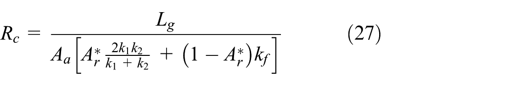
where k₁, k₂, and k_f are the thermal conductivities of the materials of the two parts and the medium, respectively. $A_r^{*}$ is the dimensionless form of the actual total contact area; $A_r^{*}=A_r/A_a$ , where A_a is the real contact area of the contact surface. L_g is the thickness of the void space at the joint. L_g = z₁ + z₂ – δ₁ – δ₂, where z₁, z₂ is the height of roughness on both sides of the joint surface, respectively. δ₁, δ₂ is the maximum deformation amount of asperity on both sides of the joint surface, respectively.

Analysis of the simulation for thermal error

Heat source analysis

Heat generation of motor

The sundry loss of servo motor is the intrinsic factor of heat generation, mainly including mechanical loss, electrical loss, magnetic loss, and additional loss. The heat generation value of a servo motor can be calculated as follows

$$Q=\frac{M_{T}n}{9550}(1-\eta )$$

(28)

where M_T is the output torque of servo motor, M_T = 65 N m; n is the motor speed, n = 3000 r/min; η is the mechanical efficiency of servo motor, η = 0.75.

Heat generation of bearing

The heat of a rolling bearing is produced by the friction between the rolling element of the bearing and the ring and the friction force caused by the lubricant; the calculation formula is

$$Q=\frac{M·n}{9550}$$

(29)

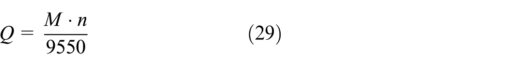
where Q is the heat generation of rolling bearings, M is the friction torque, and n is the speed of bearing, n = 3000 r/min.

For rolling bearings, the friction torque mainly includes two major categories: the friction torque M_V generated by the speed and the friction torque M_F generated by the load. Then, the total friction torque M of the bearing can be expressed as the sum of the two parts ¹⁷

$$M=M_F+M_v$$

(30)

where M_V reflects the friction loss caused by elastic hysteresis and local differential slip and can be expressed as

$$\{\begin{array}{c}\begin{array}{cc}{M}_v={10}^{-7}\times f_v{(v·n)}^{2/3}\times d_m^3\hfill & \begin{array}{cc}\hfill & v·n>2\times {10}^{-3}\hfill \end{array}\hfill \end{array}\hfill \\ \multicolumn{1}{c}{\begin{array}{cc}{M}_v=1.6\times {10}^{-5}\times f_v\times d_m^3\hfill & \begin{array}{cc}\hfill & v·n⩽2\times {10}^{-3}\hfill \end{array}\hfill \end{array}}\end{array}$$

(31)

where f_V is the empirical coefficient defined by the types and lubrication methods of bearings. The bearing adopts a single row of thrust cylindrical roller bearings and is lubricated by grease, f_V = 2; d_m is the middle diameter of bearings, d_m = 180 mm; v is the kinematic viscosity of lubricants at operating temperatures, v = 0.195 cSt.

The friction torque M_F reflects the hydrodynamic losses generated by lubricants

$$M_F=f_F·P_F·d_m^3$$

(32)

where f_F is the correlation coefficient defined by the types and load of bearings, f_F =0.0013; P_F is the calculation load of bearing friction torque, P_F =45,201N.

Friction heat of guideway

The Z-axis of large CNC gear grinding machine tools adopts a constant current hydrostatic guideway. Frictional heat is caused by sliding between slide block and guideway which can be expressed as

$$Q_s=\frac{\mu ·F_{\mathrm{s}}·v_{\mathrm{s}}}{J}$$

(33)

where Q_s is a heat guide unit of time; μ is the friction coefficient between the rails—the friction coefficient of the hydrostatic guideway is 0.0005–0.001 and the friction coefficient of the linear guide is 0.002–0.003; F_s is the rail contact load applied on the surface of the guideway, F_s = 782 N; J is the mechanical equivalent of heat; v_s is the speed of sliding relative to the guideway, v_s = 3000 mm/min.

Heat generation of the ball screw nut pair

In engineering analysis, the ball screw nut pairs are often regarded as radial thrust ball bearings subjected to a purely axial working load. Therefore, the friction heat of ball screw nut pairs can be solved by the formula of the heat quantity of the rolling bearing. The total friction torque M of the ball screw nut pair is composed of the driving torque M_D of the screw and the resistance moment M_P of the ball screw.

The driving torque M_D of the screw is the driving torque that resists the axial working load.

When the total axial load of the screw is F_a, the driving torque required to drive the nut is M_D which can be expressed as

$$M_D=\frac{F_a{P}_h}{2\pi \eta }$$

(34)

where P_h is the lead of the screw, P_h = 16 mm; η is the transmission efficiency of ball screw pair, η = 0.9; F_a = 52,780 N.

The resistance moment M_p of the ball screw is the torque required to drive the lead screw when the screw nut pair is pre-tightened and without axial load. The formula is as follows

$$M_P=\frac{F_P{P}_h}{2\pi \eta }(1-{\eta }^2)$$

(35)

where F_P is the axial preload of ball screw nut pair, F_P =18,000 N.

The total friction torque can be expressed as follows

$$M=0.94M_P+M_D$$

(36)

Heat dissipation analysis

When the fluid flows through the solid surface, convection heat transfer occurs between the fluid and the solid. Therefore, the thermal exchange in the feeding system and the external environment should be considered when thermal analysis is carried out. Convection heat transfer can be divided into natural convection heat transfer and forced convection heat transfer. The convection heat transfer mode is determined by the Grashof number G_r and the Reynolds number Re. ¹⁸ If G_r/Re² is far greater than 1, natural convection heat transfer is the dominated situation. If G_r / Re² ≈ 1, forced convection heat transfer is the dominated situation. For different convection heat transfer modes, the calculation methods of convective heat transfer coefficient are different. Therefore, before calculating the convective heat transfer coefficient, it is necessary to determine the convective heat transfer mode on the external surface of the feeding system first. The calculation method of the Grashof number G_r and Reynolds number Re is as follows

$$G_r=\frac{g\beta L^3\Delta T}{v^2},\mathrm{Re}=\frac{\rho \mathrm{uL}}{\mu }$$

(37)

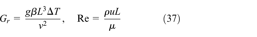
where g is the gravitational acceleration, β is the volume expansion coefficient, ΔT is the temperature difference between the fluid and solid surface, and L is the characteristic length of the structure. v, ρ, u, and μ are the kinematic viscosity, density, velocity, and kinetic viscosity of fluids, respectively.

After getting the Grashof number and Reynolds number of each outer surface, convection modes of the heat transfer on each surface can be judged. Thus, convective heat transfer coefficient of each surface can be further calculated. The formula is as follows

$$h=\frac{N_u\lambda }{L}$$

(38)

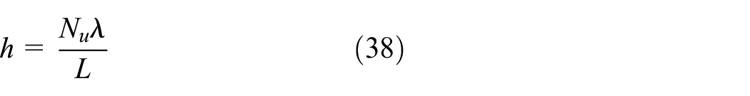
where N_u is the Nusselt number and λ is the thermal conductivity of the fluid.

Considering the equation above, convective heat transfer coefficient is related to the Nusselt number. The Nusselt number reflects the intensity of convective heat transfer. The Nusselt number in natural convection heat transfer is defined by the Prandtl constant, while the Nusselt number in forced convection heat transfer is defined by the Reynolds number.

When it comes to natural convection heat transfer, the Nusselt number is calculated by the following formula

$$N_u=0.59{(G_r·\mathrm{Pr})}^{\frac{1}{4}}$$

(39)

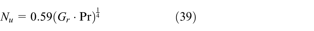
where Pr is the Prandtl constant.

When it comes to forced convection, the Nusselt number is obtained by the formula

$$\{\begin{array}{cc}{N}_u=0.326{\left(\mathrm{Re}\right)}^{0.5}\hfill & 4⩽\mathrm{Re}⩽200,000\hfill \\ \multicolumn{1}{c}{N_u=8\times {10}^{-14}{\left(\mathrm{Re}\right)}^{2.8}}& 260,000⩽\mathrm{Re}⩽320,000\hfill \end{array}$$

(40)

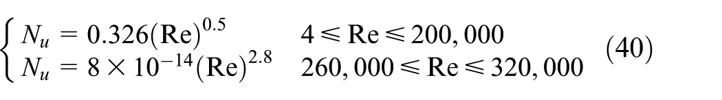
According to the formulas above, the convective heat transfer coefficient h on each outer surface can be calculated.

The convection heat transfer coefficient of the main components can be obtained, as is shown in Table 1.

Table 1.

Convective heat transfer coefficient of the main parts.

Location	Convective heat transfer coefficient (W/m2 °C)
Stationary parts (i.e. column and bearing seat)	11.2
Carriage and its upper translational parts	23.5
Rotating parts (i.e. lead screw)	67.3

The simulation for thermal error

Finite element model of the large CNC gear grinding machine tools

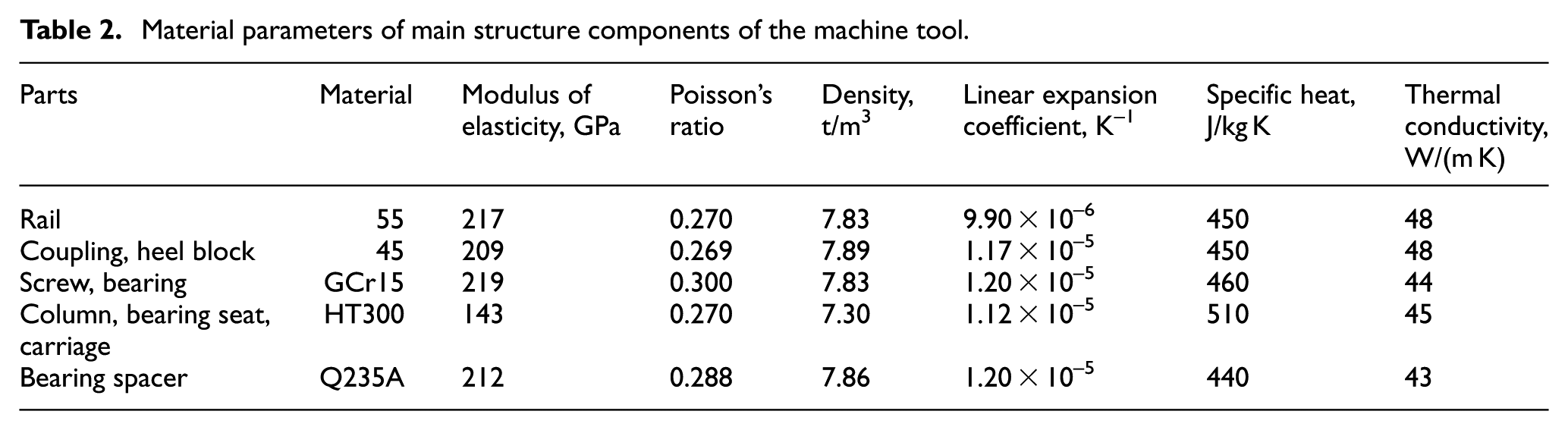
Setting up the finite element model of the large CNC gear grinding machine tools in Figure 6. Table 2 shows the material parameters of structure components of the machine tool.

Figure 6.

(a) Finite element model of the machine tool and (b) finite element mesh model of the machine tool.

Table 2.

Material parameters of main structure components of the machine tool.

Parts	Material	Modulus of elasticity, GPa	Poisson’s ratio	Density, t/m3	Linear expansion coefficient, K–1	Specific heat, J/kg K	Thermal conductivity, W/(m K)
Rail	55	217	0.270	7.83	9.90 × 10–6	450	48
Coupling, heel block	45	209	0.269	7.89	1.17 × 10–5	450	48
Screw, bearing	GCr15	219	0.300	7.83	1.20 × 10–5	460	44
Column, bearing seat, carriage	HT300	143	0.270	7.30	1.12 × 10–5	510	45
Bearing spacer	Q235A	212	0.288	7.86	1.20 × 10–5	440	43

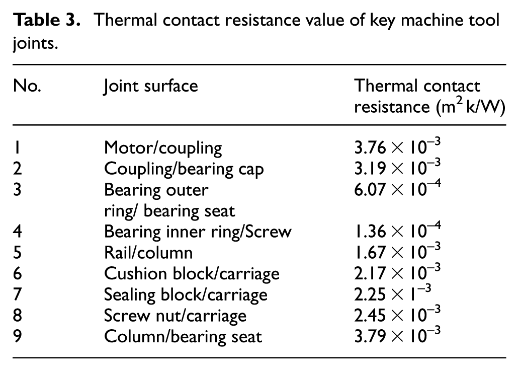
The main interfaces in the Z-axis feeding system are shown in Figure 7. In Figure 7(a), surfaces 1–4 indicate the contact surface between motor and coupling, coupling and bearing cap, bearing and bearing seat, and bearing and screw, respectively. In Figure 7(b), surfaces 1–3 indicate the contact surface between rail and column, cushion block and carriage, and sealing block and carriage, respectively. In Figure 7(c), surfaces 1–2 are the contact surface between screw nut and carriage, and column and bearing seat, respectively. Above surfaces are the contact surfaces between main heat source and other components, which will have a great influence on the heat conduction in simulation. So the TCR on the contact surface must be considered in the simulation. Table 3 lists the TCR value of key machine tool joints.

Figure 7.

The main interfaces between the parts of the Z-axis feeding system: (a) Main contact surface between the bearing seat and its surrounding part; (b) Main contact surfaces between column, rail and carriage; and (c) The contact surface between the bearing seat and the column, carriage and screw nut.

Table 3.

Thermal contact resistance value of key machine tool joints.

No.	Joint surface	Thermal contact resistance (m2 k/W)
1	Motor/coupling	3.76 × 10–3
2	Coupling/bearing cap	3.19 × 10–3
3	Bearing outer ring/ bearing seat	6.07 × 10–4
4	Bearing inner ring/Screw	1.36 × 10–4
5	Rail/column	1.67 × 10–3
6	Cushion block/carriage	2.17 × 10–3
7	Sealing block/carriage	2.25 × 1–3
8	Screw nut/carriage	2.45 × 10–3
9	Column/bearing seat	3.79 × 10–3

Finite element analysis results

The distribution of the temperature field is shown in Figure 8 when the thermal balance state is reached. Figure 9 shows the temperature field distribution of the guideway and column when the thermal balance state is reached.

Figure 8.

The temperature field distribution (a) without TCR and (b) with TCR.

Figure 9.

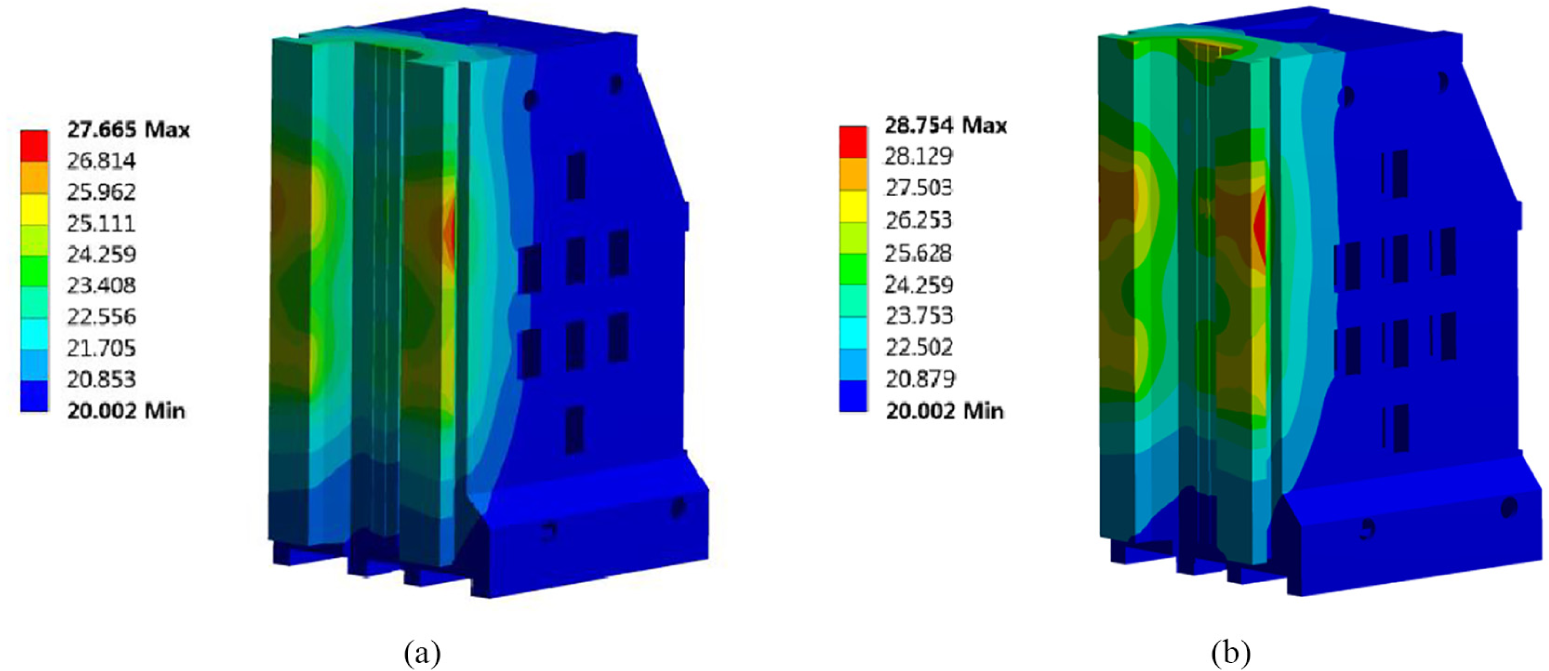
The temperature field distribution of guideway and column: (a) the temperature field distribution without TCR and (b) the temperature field distribution with TCR.

As can be seen in Figure 8, the temperature rise of the friction zone of the screw nut pair and the guideway is more obvious when the Z-axis feeding system reaches thermal steady state. The detailed temperature distribution of the hydrostatic guideway and the column is shown in Figure 9. Figures 8(b) and 9(b) are the steady-state temperature field distributions of the Z-axis feeding system and the hydrostatic guideway under the condition of TCR.

Thermal deformation analysis

To simulate the thermal deformation, the simulation results of the temperature field are applied to the finite element model of the Z-axis feeding system. Figure 10 shows the thermal deformation of the guideway when the thermal balance state is reached.

Figure 10.

The thermal deformation of the guideway: (a) the thermal deformation without TCR and (b) the thermal deformation with TCR.

Experiment

Experimental design

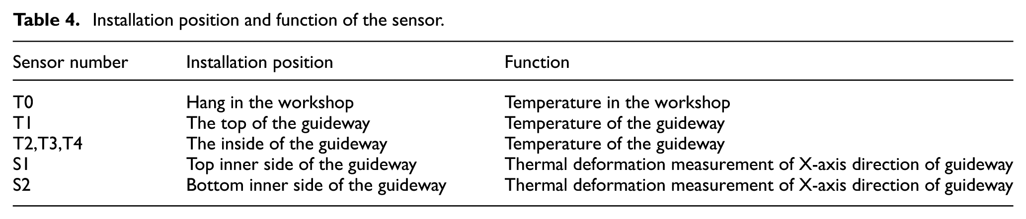
The experimental device is the Z-axis feeding system of the large CNC gear grinding machine tools in Figure 11; measuring devices and functions are as follows: the multi-function data acquisition instrument and LTS-25-02 type laser triangulation sensor were used to determine the temperature and thermal deformation. This system uses the PT100 temperature sensor to measure the temperature of the Z-axis guideway. The high-precision LTS-25-02 type laser triangulation sensor was used to collect the thermal displacement of the guideway. The acquisition frequency was once per minute. Table 4 lists the installation position and function of the sensors.

Figure 11.

The diagram of temperature and displacement sensor positions.

Table 4.

Installation position and function of the sensor.

Sensor number	Installation position	Function
T0	Hang in the workshop	Temperature in the workshop
T1	The top of the guideway	Temperature of the guideway
T2,T3,T4	The inside of the guideway	Temperature of the guideway
S1	Top inner side of the guideway	Thermal deformation measurement of X-axis direction of guideway
S2	Bottom inner side of the guideway	Thermal deformation measurement of X-axis direction of guideway

Moreover, dimensions of gear are as follows: modulus m_n is 14 mm, tooth number z_g is 81, tip diameter d_a is 1202 mm, root diameter d_f is 1139 mm, tooth width B is 180 mm, and center distance D_x is 790 mm. The Z-axis carriage motion rate is a constant speed of 3000 mm/min, the stroke of the reciprocating movement is 200 mm, and the ambient temperature of the workshop is 20 ± 0.1°C in the experiment (Figure 12).

Figure 12.

Experimental platform of thermal error.

Analysis of experimental data

The temperature measurement data of the machine tools are shown in Figure 13. In Figure 13(a)–(d), the temperature of the guideway in three cases with and without considering the TCR and the actual measurement data are shown at the points T1, T2, T3, and T4, respectively. It can be seen that the temperature of the machine tool increased rapidly in the first 4 h and the temperature increased slowly from 4 to 5 h. After 5 h, it gradually tended to the state of thermal balance. In addition, the temperature in the middle of the guideway is higher than that in the upper and lower sites, because the middle of the guideway is located in the friction zone and close to the ball screw nut pair.

Figure 13.

Temperature variation of measurement points: (a) T1, (b) T2, (c) T3, and (d) T4.

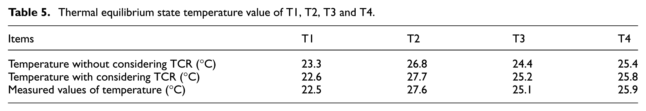
When the thermal balance was reached, the temperature of T2 and T4 reached 27.6°C and 25.9°C, respectively. The simulation results show (Figure 9) that the temperature at T2 and T4 is 26.8°C and 25.4°C when the TCR is not considered, while it is 27.7°C and 25.8°C when the TCR is considered. The temperature of T3 is slightly lower than T2 and T4, because T3 is less affected by the heat of cushion blocks. In addition, T1 lies in the non-friction zone and the heat caused by the bearing seat is reduced when the TCR is considered, so the temperature in T1 is reduced by 0.7°C. After reaching the thermal equilibrium state, T1, T2, T3, and T4 temperatures are shown in Table 5.

Table 5.

Thermal equilibrium state temperature value of T1, T2, T3 and T4.

Items	T1	T2	T3	T4
Temperature without considering TCR (°C)	23.3	26.8	24.4	25.4
Temperature with considering TCR (°C)	22.6	27.7	25.2	25.8
Measured values of temperature (°C)	22.5	27.6	25.1	25.9

In Figures 8 and 9, it can be seen that under the condition of the TCR, the overall temperature of the machine tool is higher than that without considering TCR. On the motor and the bearing seat, there are 7.1°C and 3.9°C temperature rises, and at the hydrostatic guideway, 1.1°C temperature rises. The overall temperature distribution trend is the same, but under the condition of TCR, the distribution area of the highest temperature is larger than that without considering TCR.

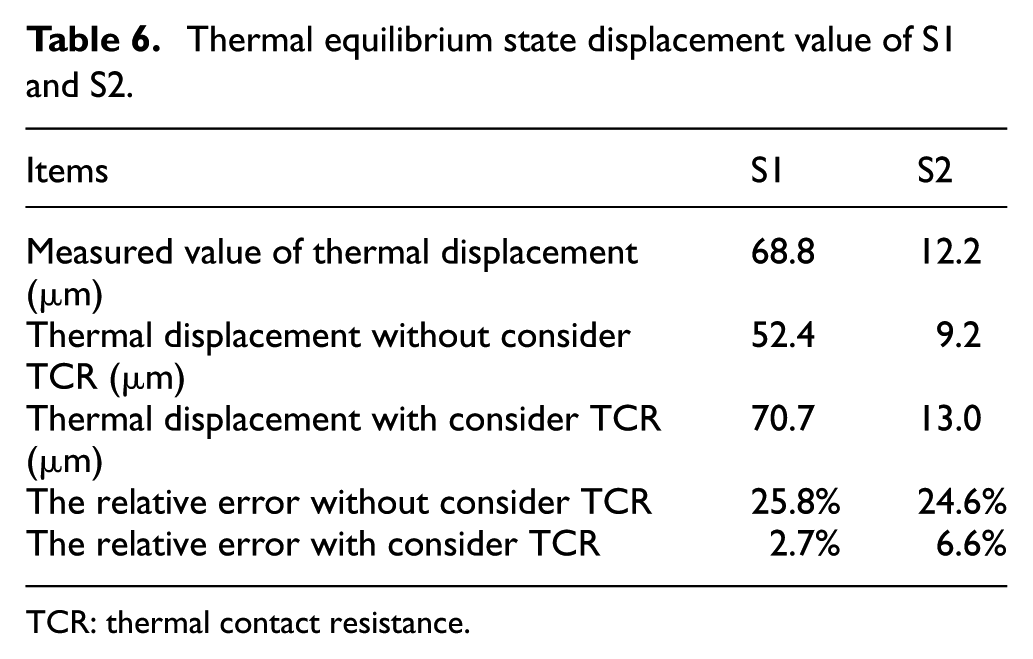
Figure 14 is the thermal displacement data of the hydrostatic guideway in the direction of X-axis. Under the effect of the thermal load, mainly tilt and pitching deformation occurred in the guideway in the X-axis direction. The deformation of the Y-axis direction and the Z-axis direction is far less than the X-axis direction, so these deformations can be ignored. It can be seen that the variation trend of the displacement was generally the same as the temperature change trend. The displacement of S1 is 68.8 μm when the state of thermal balance is reached. In the simulation results, the displacement of S1 is 52.4 μm without considering the TCR and 70.7 μm with considering the TCR. The relative errors are 25.8% and 2.7%, respectively. The S2 is located in the lower sites of the column and guideway, far away from the heat source which result in a small temperature rise and small thermal deformation. Compared with S1, the accuracy of S2 is lower when considering TCR. The experimental data of S2 are 12.1 μm. In the simulation results, the displacement of S2 is 9.2 μm without considering the TCR and 13.0 μm with considering the TCR. The relative error descends from 24.6% to 6.6%. After reaching the thermal equilibrium state, the thermal displacement of S1 and S2 is shown in Table 6.

Figure 14.

Displacement variation of measurement points: (a) S1 and (b) S2.

Table 6.

Thermal equilibrium state displacement value of S1 and S2.

Items	S1	S2
Measured value of thermal displacement (μm)	68.8	12.2
Thermal displacement without consider TCR (μm)	52.4	9.2
Thermal displacement with consider TCR (μm)	70.7	13.0
The relative error without consider TCR	25.8%	24.6%
The relative error with consider TCR	2.7%	6.6%

TCR: thermal contact resistance.

In Figure 10, the thermal deformation trend of the guideway was roughly similar whether the TCR is considered or not. The guideway produced the tilted and pitching deformation in the direction of the X-axis; the maximum displacement is 55.181 and 72.991 μm, respectively. The displacement of the model is greater when considering the TCR because of the higher temperature. The results show that the temperature value and thermal error obtained by this method are in good agreement with the experimental data.

Conclusion

In this article, the theoretical calculation and numerical analysis of the thermal error in the Z-axis feeding system of large CNC gear grinding machine tools are carried out. The thermal error of the Z-axis guideway in the processing state is obtained using the FEM. Compared with the traditional FEM, this method has higher accuracy and reliability when considering the TCR:

1. Based on the fractal theory, the W-M fractal function and Hertz theory are used to analyze the deformation state and contact state of the asperities on the machine tool joint surface. The actual contact area of joint surface is obtained which is used to calculate the TCR on the joint surface. In addition, the surface fractal parameters are obtained using the RMSM method.

2. A comprehensive finite element model is established to conduct transient thermal-structural interactive analysis of Z-axis feeding system with consideration of the TCR, internal heat source, and convective heat transfer coefficients. The difference in temperature and thermal deformation of the guideway is analyzed when the TCR is taken into consideration or not.

3. An experimental platform of machine tool temperature and thermal error is established to verify the accuracy and reliability of the theoretical and simulation models. Then, the temperature and displacement of the guideway are measured and analyzed. The results show that the relative error of S1 is less than 2.7% and that of S2 is less than 6.6% by comparing the measured values of the thermal displacement with simulated values of the thermal displacement.