Sage Journals: Discover world-class research

Abstract

Micron droplet deposition onto a wall in an impinging jet is important for various applications like spray cooling, coating, fuel injection, and erosion. The impinging process is featured by abrupt velocity changes and thus complicated behaviors of the droplets. Either modeling or experiment for the droplet behaviors is still challenging. This study conducted numerical modeling and compared with an existing experiment in which concentric dual-ring deposition patterns of micron droplets were observed on the impinging plate. The modeling fully took into account of the droplet motion in the turbulent flow, the collision between the droplets and the plate, as well as the collision, that is, agglomeration among droplets. Different turbulence models, that is, the v²−f model, standard k–ε model, and Reynolds stress model, were compared. The results show that the k–ε model failed to capture the turbulent flow structures and overpredicted the turbulent fluctuations near the wall. Reynolds stress model had a good performance in flow field simulation but still failed to reproduce the dual-ring deposition pattern. Only the v²−f model reproduced the dual-ring pattern when coupled with droplet collision models. The results echoed the excellent performance of the v²−f model in the heat transfer calculation for the impinging problems. The agglomeration among droplets has insignificant influence on the deposition.

Keywords

Micron droplets deposition impinging jet collision agglomeration

Introduction

Micron droplet deposition on solid surface plays important roles in various applications, such as spray cooling, coating, and fuel injection.^1,2 A comprehensive modeling for these processes is still challenging due to the limited understanding about the flow structures near the wall, the agglomeration among the droplets, and the collisions between droplets and the wall. The impaction of droplets larger than 20 µm in diameter has been extensively studied.^3,4 There is a lack of investigation for droplet of about 1 µm since it is difficult in experiment to observe in situ.² Among the few studies, Liu et al.² observed the deposition patterns of droplets of about 1 µm and found a dual-ring deposition pattern on the wall.

Numerical methods, that is, direct numerical simulation (DNS), large eddy simulation (LES), and Reynolds-averaged Navier–Stokes (RANS) models, have been employed to simulate turbulent flow structures of impinging jet.^5,6 DNS is most straightforward and provides precise results up to the smallest Kolmogorov scale. However, both DNS and LES are expensive in computational cost, which makes them rarely applicable for industrial applications especially in high Reynolds number (Re) cases.⁷ Klein et al.⁸ and Hattori and Nagano⁹ used DNS to simulate impinging jet when the Re was lower than 10,000. Tsubokura et al.¹⁰ applied both DNS and LES to predict a three-dimensional impinging jet, and the Re was 2000 for the DNS simulation and 6000 for LES.

Regarding the droplet collisions, the Lagrangian discrete phase model has been employed for dilute case.^7,11,12 Droplet–droplet collisions and droplet–wall interaction are complicated.^13,14 A stochastic approach for droplet collisions with a probability-based algorithm was proposed by O’Rourke, which has been widely used in droplet collision simulations.¹⁵ However, this method is time-consuming and manifests mesh dependency because collisions are supposed to happen in the same cell.^16–18 Zhang et al.¹⁸ proposed a mesh-independent model considering the collisions in different cells to solve the problems of O’Rourke’s model. For turbulence-induced agglomeration of fine particles, fictitious collision partners were used by Oesterle and Petitjean¹⁹ and Sommerfeld.²⁰ Xu et al.²¹ raised an industry-scale turbulence agglomeration model for fine particle based on Zhang et al.’s mesh-independent work. Xu et al.’s²¹ model searched for real collision pairs with turbulent collision kernels to get the collision frequencies.

In this work, the deposition of liquid droplets onto a wall in an impinging turbulent air jet was simulated. The flow structures of the confined turbulent air jet flow were analyzed and the relationships between the flow filed and the deposition position of the droplets were shown. Three different turbulence models, that is, the v²−f model,^22,23 standard k−ε model,²⁴ and Reynolds stress model (RSM),^25,26 were applied and the results of deposition were compared to the experiment.

Governing equations

Droplets were treated as discrete phase, and Eulerian–Lagrangian approach was used. For the gas flow, the incompressible Navier–Stokes equations were solved to get the flow structures. The solution variables in the exact Navier–Stokes equations were decomposed into two parts, that is, the time-averaged part and the fluctuating part. Equations (1) and (2) are the Cartesian tensor form of RANS equations, in which the velocities and other variables represent the time-averaged values

\frac{\partial ρ}{\partial t} + \frac{\partial}{\partial x_{i}} (ρ u_{i}) = 0

(1)

\frac{\partial}{\partial t} (ρ u_{i}) + \frac{\partial}{\partial x_{i}} (ρ u_{i} u_{j}) = - \frac{\partial p}{\partial x_{i}} + \frac{\partial}{\partial x_{j}} [μ (\frac{\partial u_{i}}{\partial x_{j}} + \frac{\partial u_{j}}{\partial x_{i}} - \frac{2}{3} δ_{ij} \frac{\partial u_{l}}{\partial x_{l}})] + \frac{\partial}{\partial x_{j}} (- ρ \bar{{u'}_{i} {u'}_{j}})

(2)

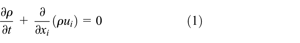
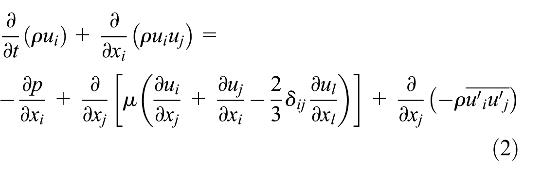
where ρ is the density of the fluid, t is the time, µ is the dynamic viscosity, and u is the turbulent components of velocity. Subscript i stands for the component of x direction, and j for the component of y direction. δ_ij is the Kronecker delta, which means that if i = j, δ_ij = 1, if i ≠ j, δ_ij = 0.

In equation (2), the Reynolds stresses $- ρ \bar{{u'}_{i} {u'}_{j}}$ are expressed by different turbulence models. A common method was to relate the Reynolds stresses to the mean velocity based on Boussinesq hypothesis, which was applied in standard k–ε model. Standard k–ε model has been applied widely in engineering since it needs low computational cost to calculate the turbulent viscosity. However, it assumes that the turbulent viscosity is an isotropic scalar quantity which may not suit for near-wall region. The v²−f model takes the near-wall turbulence anisotropy into consideration. The eddy viscosity is evaluated by the velocity scale, v², instead of the turbulence kinetic energy. The RSM abandons the isotropic eddy-viscosity hypothesis to overcome standard k–ε model’s weakness. The RSM solves the transport equation of Reynolds stresses and an equation of dissipation rate. The computational cost for RSM is higher than standard k–ε model and v²−f model.

Droplets are treated as discrete phase and they exchange momentum, mass, and energy with the fluid phase. In our cases, the volume fraction of droplet is less than 0.01%. The volume fraction is neglected in simulation as well as the rotation of droplets. The trajectories of droplets are calculated in a Lagrangian reference frame by integrating the forces on the droplets

\frac{d {\vec{u}}_{d}}{dt} = F_{D} (\vec{u} - {\vec{u}}_{d}) + \frac{\vec{g} (ρ_{d} - ρ)}{ρ_{d}} + \vec{F}

(3)

where ${\vec{u}}_{d}$ is the velocity of droplet, $\vec{u}$ is the velocity of fluid, $\vec{g}$ is the gravity, ρ_d is the density of the droplet, ρ is the density of the fluid, and t is the time. $F_{D} (\vec{u} - {\vec{u}}_{d})$ is the drag force (force/unit droplet mass) and can be expressed as²⁷

F_{D} = \frac{18 μ}{ρ_{d} d_{d}^{2}} \frac{C_{D} Re}{24}

(4)

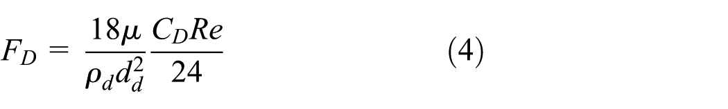
where µ is the molecular viscosity of the fluid, and d_d is the droplet diameter. Re is the relative Reynolds number based on the diameter of the droplets and the relative velocity between fluid and the droplet. For micron droplets, C_D = a₁ + a₂/Re + a₃/Re², where a₁, a₂, and a₃ are constants that apply over several ranges of Re given by Morsi and Alexander.²⁷ For sub-micrometer droplets, Stokes–Cunningham Drag Law is proved to be valid.^28,29 Considering that the droplet size in this study is larger than 0.5 µm, spherical drag law is applied instead of Stokes–Cunningham Drag Law.²⁷ $\vec{F}$ is an additional acceleration force. Xu et al.³⁰ proved that for fine droplets, Brownian force was important, while virtual mass force, Basset history force, Saffman force, and Magnus force could be negligible. Brownian motion was an important reason for the collisions between fine droplets. A parcel-based stochastic collision model was used to calculate the droplet collision rate. The inter-particle collision frequency depends on the kinetic theory of the gases by the following equation

f_{c} = \frac{n π {(r_{1} + r_{2})}^{2} v_{rel}}{V_{c}} = n_{p} π {(r_{1} + r_{2})}^{2} v_{rel} = n_{p} K

(5)

where r₁ and r₂ are the radii of the particles, v_rel the relative velocity of two particles, and n_p = n/V_c the particle number density in the respective control volume. K is defined as the collision kernel. The collision kernel K considering Brownian motion and the turbulent effect is

K^{2} = K_{Brownian}^{2} + K_{turb}^{2}

(6)

In this study, Brownian motion-induced collision kernel is given by Otto et al.³¹

K_{Brownian} = \frac{2 k_{b} T}{3 μ_{f}} (\frac{1}{r_{1}} + \frac{1}{r_{2}}) (r_{1} + r_{2})

(7)

where k_b is Boltzmann constant. For details of the turbulent collision kernels, see Xu et al.²¹

Results and discussion

Free jet flow

At first, a free jet flow without droplets was simulated to have an idea about the performance of the different turbulence models. Simulation results were compared with the experimental result by Liu et al.² They used a hot-wire probe to measure the flow characteristics of the free jet. The diameter of the jet nozzle was 9.5 mm. The jet exit velocity was 30 m/s, and the Reynolds number based on the exit diameter was 19,300.

Three models were carried out to simulate the free jet flow, that is, the k–ε model, v²−f model, and RSM. The standard k–ε model is based on transport equations for the turbulence kinetic energy, k, and its dissipation rate, ε. A basic assumption is that the flow is fully turbulent, and the effects of molecular viscosity can be neglected. The v²−f model is a four-equation model, and the transport equations are based on the kinetic energy k, its dissipation rate ε, a velocity variance scale $\bar{v^{2}}$ , and an elliptic relation function f. The v²−f model has been proved valid without the aid of wall equation in impinging problem.²³ The RSM accounts for the anisotropy of the turbulence, working well for swirl and rotation complex flows.

Figure 1 shows the mean velocity profiles normalized by the local maximum velocity at different streamwise locations: (a) z/D = 1, (b) z/D = 2, and (c) z/D = 3. The simulation results of the k–ε model, v²−f model, and RSM all well agreed with the experimental results.

Figure 1.

Performance of different models on flow field simulation: normalized velocity profile at different streamwise positions: (a) z/D = 1, (b) z/D = 2, and (c) z/D = 3. D is the nozzle diameter, z the streamwise direction, and r the radial direction.

The turbulence intensity results, however, were different for different models. As shown in Figure 2, the normalized turbulence intensity at different streamwise locations was compared with the experimental results. The k–ε model always overpredicted, the RSM had better, and the v²−f model had the best agreement with the experiment. For standard k–ε model, the assumption is that the flow is fully turbulent and the effects of molecular viscosity are negligible. The Boussinesq hypothesis is also employed which means the turbulent viscosity is an isotropic scalar quantity. Therefore, the model is only valid for fully turbulent flows, where the turbulence anisotropy is not obvious and the molecular viscosity is small enough.⁷ In our case, the turbulence of the jet flow is not high enough near solid wall and the turbulence is anisotropic there. Standard k–ε model is therefore not suitable.

Figure 2.

Performance of different models on flow field simulation—normalized turbulence intensity at different streamwise positions: (a) z/D = 1, (b) z/D = 2, and (c) z/D = 3.

Behnia et al.²² have employed v²−f model for impingement heat transfer simulation which was an unconfined impinging jet onto a flat plate at Re = 23,000. They found that the k–ε model overpredicted the heat transfer rate in the stagnation region by about 100%, while the v²−f model reproduced the experiments fairly well. According to the v²−f model results in Figure 2, the turbulence intensity at the centerline, that is, r = 0, was around 5%, which means the turbulent fluctuation was not negligible. The turbulence intensity in the shear layer was 15%, which indicates that the flow in exit shear layer is fully turbulent.

Impinging jet with droplets

According to the above section, the v²−f model had the best simulation for the free jet flow with a moderate computation cost. In this section, the impinging jet was simulated together with droplets. The geometry of the impinging jet system, the property of the droplet, and the boundary conditions were set according to the experiments in Liu et al.’s² work. Figure 3 shows the schematic representation of the simulation jet setup. The simulation system was of two-dimensional axial symmetry. The diameter of the jet nozzle was 9.5 mm; the diameter of the plate was 100 mm. The distance between the jet nozzle and the plate was 10 mm; the distance between the droplet inlet and the jet nozzle was 50 mm.

Figure 3.

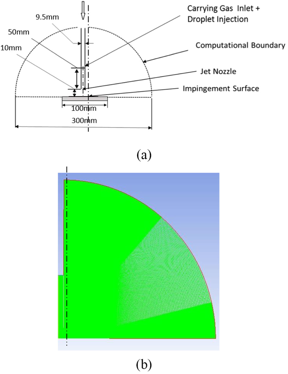
Simulation schematic representation of the impinging jet with micron and submicron droplets: (a) geometry and boundary conditions and (b) mesh setup.

According to the experiment,² the droplets were set as olive oil with the density ρ = 920 kg/m³, the surface tension σ = 3.2 × 10⁻² N/m, and the viscidity µ = 8.1 × 10⁻² Ns/m². The system temperature was 298 K. The size distribution of the inject droplets is shown in Figure 4. The figure indicates that most of the droplets were smaller than 2 µm. The number concentration of the droplets at the exit was 1.94 × 10¹³/m³.

Figure 4.

Size distribution of the inject droplets at the inlet according to the experiment.²

The boundary conditions of the simulation were set as follows. The inlet was a velocity inlet with an average velocity of 30 m/s. The outer boundaries of the simulation domain were set as pressure outlet for the fluid and set as escape condition for the droplets. Mundo et al.’s study showed that for droplets with diameters smaller than 10 µm, the critical velocity to rebound was more than 30 m/s.⁴ So the plate was set as a trap condition for droplets, which means the droplets will not rebound.

Figure 3(b) is a sketch of the mesh setup with a non-uniform mesh of 202,507 quadrilateral cells. The mesh independence has been confirmed by refining the mesh by 1.5 times in both axial and radial directions. FLUENT was used with double precision considering the length–width ratio of the mesh near the wall and the discrete parcel model. The spatial discretization of gradient was least squares cell-based scheme. The spatial discretization of turbulence kinetic energy, turbulence dissipation rate, velocity variance scales, and elliptic relaxation function was the third order. The first grid point was at y⁺ ≈ 1 or less when using the v²−f model and RSM. Figure 5 shows the y⁺ distribution of different models in the first grid.

Figure 5.

y⁺ distribution in the v²−f model and RSM on the wall.

A discrete random walk (DRW) model was applied to simulate the stochastic motion of the droplets due to turbulence. The DRW model is a stochastic model to calculate the instantaneous fluid velocity. The fluctuating velocity components are discrete piecewise constant functions of time. Turbulence-induced collision in the case could be important. In this simulation, a mesh-independent turbulent collision model was applied by user-defined function (UDF). For details, see Zhang et al.¹⁸ and Xu et al.²¹.

Figure 6 shows the simulation results and the comparison to the experiment about the droplet deposition pattern on the plate in terms of the normalized thickness distribution. The deposition thickness values at the stagnation point were used for the normalization. An important result in the experiment was that there were two peaks on the plate that looked like concentric dual-ring pattern as marked in Figure 6. For the simulation results, the v²−f model also got the two peaks, which agreed with the experiment qualitatively. In the experiment, the position of the first peak was at around r/D = 0.7 and the second one at r/D = 1.7. In the simulation, the position of the first peak was at around r/D = 0.6 and the second one at r/D = 2.7. In contrast, the RSM only obtained one peak and the single peak was great in magnitude, indicating that the droplet deposition was highly localized, which was quite different from the experiment.

Figure 6.

Normalized thickness distribution of deposited droplets on the plate, comparison between simulations and the experiment. The experiment and the v²−f model got two peaks, that is, dual-ring pattern, while the RSM only obtained one peak.

The results of velocity magnitude distribution of v²−f model and RSM were compared in Figure 7(a). The results were seen similar for the two models, which cannot explain why the RSM did not get the two deposition peaks as v²−f model did. For both models, there was a stagnation point in the center of the plate, and the velocity reached its peak at around r/D = 2. The results of the turbulence kinetic energy distribution were then compared as shown in Figure 7(b). For both models, the turbulence energy was low at the stagnation point, in agreement with Behnia et al.’s²³ experiment. The local heat transfer coefficient was increased with the local turbulence kinetic energy.^2,23 However, the differences were apparent that for v²−f model, the turbulence kinetic energy was concentrated along the plate in a long range, while for the RSM the energy concentration quickly left the plate which could be the reason the RSM did not produce as many deposition peaks as v²−f model did. An even more straightforward evidence was shown in Figure 7(c) about the dynamic pressure distribution on the plate. The dynamic pressure on the wall was due to the normal component of fluid velocity near the plate. It was clear that the v²−f model produced a series of peaks and the biggest two of them were located at r/D = 0.9 and 3, respectively, about corresponding to the two droplet deposition peaks. For the RSM, the dynamic pressure is much weaker. It was concluded that the flow field in the v²−f model was more favorable for droplet deposition. The accuracy of RSM could be limited by the closure assumptions that are used to model various terms in the exact transport equations for the Reynolds stresses.²⁵

Figure 7.

Comparison of RSM and the v²−f model results on (a) the velocity magnitude distribution, (b) the turbulence kinetic energy distribution, and (c) the dynamic pressure on the plate. The result of the RSM is on the left and the v²−f model is on the right for (a) and (b).

Conclusion

This study conducted numerical modeling and compared with an existing experiment in which concentric dual-ring deposition patterns of micron and submicron droplets were observed. Different turbulence models, that is, the v²−f model, standard k–ε model, and RSM, were compared. The two basic assumptions for standard k–ε model, that is, the negligible effects of molecular viscosity and the isotropic eddy viscosity,²⁴ make the standard k–ε model not suitable for injection and impinging jet process simulation. RSM had a good performance in flow field simulation but still failed to reproduce the dual-ring deposition pattern. Only the v²−f model reproduced the dual-ring pattern when it was coupled with droplet collision models, which is in agreement with previous Zuckerman and Lior’s³² work which made a comparison of different turbulence models, that is, k–ε, k–ω, Realizable k–ε, RSM, v²−f, and LES, for impinging jet problem and proved that v²−f had advantages in the computation cost and accuracy in heat transfer coefficient prediction.

Footnotes

Handling Editor: Kai Bao

Declaration of conflicting interests

The author(s) declared no potential conflicts of interest with respect to the research, authorship, and/or publication of this article.

Funding

The author(s) disclosed receipt of the following financial support for the research, authorship, and/or publication of this article: This work was supported by National Key R&D Program of China, No. 2016YFB0600605, and National Natural Science Foundation of China, No. 51622601.

ORCID iD

Hao Wang

References

Jambunathan

Lai

Moss

et al . A review of heat transfer data for single circular jet impingement. Int J Heat Fluid Fl 1992; 13: 106–115.

Liu

Nink

Merati

et al . Deposition of micron liquid droplets on wall in impinging turbulent air jet. Exp Fluids 2009; 48: 1037–1057.

Andreassi

Ubertini

Allocca

Experimental and numerical analysis of high pressure diesel spray–wall interaction. Int J Multiphas Flow 2007; 33: 742–765.

Mundo

Sommerfeld

Tropea

Droplet-wall collisions: experimental studies of the deformation and breakup process. Int J Multiphas Flow 1995; 21: 151–173.

Jaramillo

Trias

Gorobets

et al . DNS and RANS modelling of a turbulent plane impinging jet. Int J Heat Mass Tran 2012; 55: 789–801.

Satake

Kunugi

Direct numerical simulation of an impinging jet into parallel disks. Int J Numer Method H 1998; 8: 768–780.

Tian

Ahmadi

Particle deposition in turbulent duct flows—comparisons of different model predictions. J Aerosol Sci 2007; 38: 377–397.

Klein

Sadiki

Janicka

Investigation of the influence of the Reynolds number on a plane jet using direct numerical simulation. Int J Heat Fluid Fl 2003; 24: 785–794.

Hattori

Nagano

Direct numerical simulation of turbulent heat transfer in plane impinging jet. Int J Heat Fluid Fl 2004; 25: 749–758.

10.

Tsubokura

Kobayashi

Taniguchi

et al . A numerical study on the eddy structures of impinging jets excited at the inlet. Int J Heat Fluid Fl 2003; 24: 500–511.

11.

Berlemont

Chang

Gouesbet

Particle Lagrangian tracking with hydrodynamic interactions and collisions. Flow Turbul Combust 1998; 60: 1–18.

12.

Salmanzadeh

Rahnama

Ahmadi

Particle transport and deposition in a duct flow with a rectangular obstruction. Particul Sci Technol 2007; 25: 401–412.

13.

Meyer

Deglon

Particle collision modeling—a review. Miner Eng 2011; 24: 719–730.

14.

Heinl

Bohnet

Calculation of particle–wall adhesion in horizontal gas–solids flow using CFD. Powder Technol 2005; 159: 95–104.

15.

O’Rourke

PJ.

Collective drop effects on vaporizing liquid sprays. Princeton, NJ: Princeton University, 1981.

16.

Schmidt

Rutland

A new droplet collision algorithm. J Comput Phys 2000; 164: 62–80.

17.

Cai

et al . Droplet collision and coalescence model. Appl Math Mech 2006; 27: 67–73.

18.

Zhang

Wang

A new mesh-independent model for droplet/particle collision. Aerosol Sci Tech 2012; 46: 622–630.

19.

Oesterle

Petitjean

Simulation of particle-to-particle interactions in gas solid flows. Int J Multiphas Flow 1993; 19: 199–211.

20.

Sommerfeld

Validation of a stochastic Lagrangian modelling approach for inter-particle collisions in homogeneous isotropic turbulence. Int J Multiphas Flow 2001; 27: 1829–1858.

21.

Shen

Wang

An industry-scale modeling for the turbulence agglomeration of fine particles. Adv Mech Eng 2015; 7: 1–10.

22.

Behnia

Parneix

Durbin

PA.

Prediction of heat transfer in an axisymmetric turbulent jet impinging on a flat plate. Int J Heat Mass Tran 1998; 41: 1845–1855.

23.

Behnia

Parneix

Shabany

et al . Numerical study of turbulent heat transfer in confined and unconfined impinging jets. Int J Heat Fluid Fl 1999; 20: 1–9.

24.

Chen

Comparison of different k-ε models for indoor air flow computations. Numer Heat Tr B-Fund 1995; 28: 353–369.

25.

Launder

Reece

Rodi

Progress in the development of a Reynolds-stress turbulence closure. J Fluid Mech 1975; 68: 537–566.

26.

Launder

BE.

Second-moment closure and its use in modelling turbulent industrial flows. Int J Numer Meth Fl 1989; 9: 963–985.

27.

Morsi

Alexander

AJ.

An investigation of particle trajectories in two-phase flow systems. J Fluid Mech 1972; 55: 193–2080329.

28.

Davies

CN.

Definitive equations for the fluid resistance of spheres. P Phys Soc 1945; 57: 259.

29.

Ounis

Ahmadi

McLaughlin

JB.

Brownian diffusion of submicrometer particles in the viscous sublayer. J Colloid Interf Sci 1991; 143: 266–277.

30.

Zhang

Wang

et al . Fine particle behavior in the air flow past a triangular cylinder. Aerosol Sci Tech 2013; 47: 875–884.

31.

Otto

Fissan

Park

et al . The log-normal size distribution theory of Brownian aerosol coagulation for the entire particle size range: part II—analytical solution using Dahneke’s coagulation kernel. J Aerosol Sci 1999; 30: 17–34.

32.

Zuckerman

Lior

Jet impingement heat transfer: physics, correlations, and numerical modeling. Adv Heat Trans 2006; 39: 565–631.

Numerical simulation of micron and submicron droplets in jet impinging

Abstract

Keywords

Introduction

Governing equations

Results and discussion

Free jet flow

Impinging jet with droplets

Conclusion

Footnotes

Declaration of conflicting interests

Funding

ORCID iD

References