
Abstract
Although the bus probe data have been widely adopted for examining the transit route efficiency, this application cannot guarantee the accuracy in special temporal and spatial segments due to the inadequate probe samples. This study evaluates the feasibility of automatic vehicle location data as probes for the bus route travel time evaluation. Our techniques explore the minimum requirement of transit automatic vehicle location data to recover the bus trajectories in various spatial–temporal dimensions along the scheduled transit routes. First, a three-dimensional tensor is established to infer the uncovered link traveling information in current time slots and the last short-term period. Then, a general form is proposed to calculate the local mean travel speed and the average link travel time in each separated time slot of day. Finally, a case study has been conducted using field transit automatic vehicle location data running on a bus route corridor in Edmonton, Canada. The results demonstrate the effectiveness and efficiency of low-frequency bus automatic vehicle location data as probes for transit route efficiency measurement by comparing with baseline approaches. This work also supports the feasibility of using automatic vehicle location–equipped buses as customized buses for choosing alternate path based on evaluating the current transit efficiency on all routes.
Keywords
Introduction
Estimation of bus travel speed and travel time provides important functions for transit service agencies to determine the performance of its units of operations and further improve the schedule, route plan, on-arrival reliability, and so on. Lots of solutions have been proposed for real-time vehicle speed and travel time estimations, for example, microwave detectors, radar detectors, camera sensors, and other devices deployed at fixed detecting locations. 1 However, road segments have not been completely equipped with detecting sensors due to the increasing cost, and thus the range of these measurements is very limited. 2 Probe vehicle global positioning system (GPS) data are regarded as one of the most alternative methods for transit travel time applications, especially recently when transit vehicles are increasingly equipped with automatic vehicle location (AVL) for recording the bus positions when traveling the route, which in turn provides a novel type of sensor for travel speed and travel time estimation purposes. Unlike the probe samples obtained from other sources, such as taxis, the transit buses are keeping apprised of routes and schedules, and thus it enables a practical measurement of speed and travel time between two explicit locations.
Although the use of bus AVL sample data as probes creates a potential solution for practical implementation for obtaining the transit travel speed and travel time of any route segment where buses equipped with GPS system are active, the technique has not yet been well solved given the following challenges: (1) road segments are timely traveled by transit buses on scheduled time slots, which creates difficulties for examining the link segment travel time for each fraction in time slots set, such as from 2:00–4:00, and the sample size reduced significantly on each link; (2) the frequency of transit AVL samples is designed to be less than two per minute, and the AVL system has error and missing records when the GPS devices lost the accuracy, which creates difficulties in inferring the truly traversed path between two reported positions. These issues limit the usage of transit probes and therefore need more sophisticated methods for processing and recovering the missed transit samples.
In this article, we proposed a general model for estimating the transit local time-mean travel speed and average link travel time based on bus AVL samples. Our technique estimates the transit travel speed field information on consequent sections along the bus route corridor in different time slots by constructing a three-dimensional (3D) tensor, which infers the missing speed information using traversed bus trajectory samples in contemporary time slots and over the past time slots, as well as road network data. The contribution of this article is to estimate the dynamic bus time–space travel speed and travel time information on scheduled transit routes by reconstructing and allocating the individual transit trajectories into the temporal–spatial speed field. Our study also demonstrates that the low-frequency transit probes can contribute to the data source for effective travel time applications at minimum cost.
The remainder of this article is organized as follows: first, the most recent related studies were summarized and reviewed. Then, a general prescription was presented for identifying the set of calculations that are needed to implement the transit route travel time estimation. This is followed by the sections presenting a case study, results and discussions, and conclusions.
Literature review
The investigation of travel speed and travel time application using a probe vehicle has been recently conducted increasing technical attention by researchers to implement more practical traffic applications. 2 However, the most significant problem existed with the sparse sample size and low sampling frequency, which lead to difficulties when using probe samples to explore the traversed segments between sequential logger points. Especially in urban arterial area, low probe sampling frequency creates challenges in inferring the vehicle-traversed route in the network, which may involve more than two paths between two recorded GPS locations.3–5
Considerable research on travel speed and travel time applications in an urban area is mostly focused on improving the estimation performance using low-frequency GPS probes, network geographic information, and other attributes. For example, Jenelius and Koutsopoulos 3 proposed a model to integrate the network patterns and historical traffic data, and then examined the traffic flow on explicit road segments and the traffic delay at signalized intersections. The model can be resolved practically by the maximum likelihood estimation method. Fabritiis et al. 6 improved the link travel speed estimation by considering the traffic patterns on the neighboring links, which have a short-term effect on the traffic status of the current segment. But the model increases the complexity and instability when scaling up to a large network area. In addition, the sparsity of the probe sample size, that is, consecutive links are not completely covered by probes in each time slot, is a common issue limiting the usage of the model. Cathey and Dailey 7 investigated individual transit bus probe to estimate the travel speed based on Kalman filter algorithm, which in turn provided the space-mean travel speed and link travel time information. However, the proposed method is only testified using high-frequency probe data.
Other methods in terms of route travel time estimation involved the allocation of travel time to each segment. Hellinga et al. 8 divided the link travel time into three components: free flow travel time, stopping time at traffic signals, and delay due to link congestion. If there are traffic signal devices along the link, the traffic signal–related delay would be more likely to occur and estimated based on a probability function. In large-scale network applications, the observation of probe travel time was decomposed into each traversed route segment.9–13 Zheng and van Zuylen 14 inferred the travel time information of probe vehicle on traversed links by an improved multi-layer artificial neural network (ANN) model. Chakroborty and Kikuchi 15 collected transit probe data on urban corridors to evaluate the sample size and data quality on each segment and demonstrate the possibility of using the transit probe data source for the traffic monitoring purposes.
Although the state-of-the-art technologies have been developed and the valuable usage of bus GPS data for various travel speed and travel time applications has been clearly testified, there are several issues remaining unresolved in the existing studies. On the one hand, the large scale of travel time estimation has minimum requirement for the probe sample size deployed along the entire route in each time slot. 16 The average historical link travel time cannot accurately represent the current situations when the traffic dynamic is complicated. On the other hand, the influence of the traffic patterns of the neighboring links on the sparse sample’s travel speed and travel time on individual segment has not been testified with dependent relationship, which may lead to uncertainty of travel time estimation in variable traffic situations. 17
Methodology
In this section, we set up a general scheme for transit route travel speed and travel time estimation based on bus AVL records. In Figure 1, an algorithm framework is presented by three major processes, the detailed variables and notations on the major components and data attributes of which are represented by a vector

Overall framework for transit route travel time estimation.
First, we project the bus AVL raw data (presented in the longitude and latitude format) into the referred geographic road network by applying path inference and map matching algorithm.
18
Based on these processed sample data, the probe vehicle’s traveling information can be investigated on separated links at different times of a day. Then, a 3D tensor
Trip inference
The transit AVL system reports the real-time vehicle locations based on the vehicular GPS devices. However, these raw probe data cannot be directly used for travel time application due to the lack of route length between two probe positions, and thus it is supposed to transform the original sample data into road mapped samples, which is not widely provided by the transit AVL system. In this section, the trip inference algorithm is applied to extract the trip of each individual along the traversed route, as shown in Figure 2.

Definition of road network and path shape points.
In Figure 2, there is a sample pattern plotted in a map of 23 Ave., Edmonton, Canada. The distance-into-geodetic path is described to be the travel distance–related information. Given the vehicle AVL data and road network data, we can use path inference algorithm to determine the transit route trip and a vehicle traveling distance-into-trip. Then, a set of generic definitions are necessary to accomplish the task of the path inference. In Figure 2, the notations are defined as follows:
Definition 1: probe sample. A probe sample
Definition 2: path point interval (PPI). PPI is a dataset of stretched road distance between the successive connected reference points, which represent the geographical features (start points, end points, and points at the curve sections) of a path.
Definition 3: probe trip. Probe trip is a group of processed probe samples matched with a set of traversed PPI, for example,
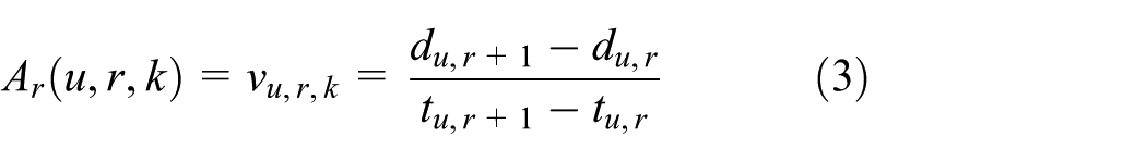
Definition 4: link travel speed. The parameter
The transit AVL system produces real-time reports of vehicle identifier, timestamp, and vehicle location (longitude and latitude). However, most of the applications using the transit probe data require the vehicle’s location information to be directly related to the distance-into-geodetic path, which assign the spatial–temporal transit probe samples to the scheduled route locations and time slots. Figure 3 depicts the procedure of the trip inference algorithm, which consists of two steps: map matching and path inference. The function of map matching is projecting the probe GPS records into the corresponding geographical road pattern, in order to obtain the probe’s traveling distance in the field path. It is challenged to infer the matched points into the correct candidate links when the transit route is surrounded by several approached links i.e., the practical GPS position may be measured at the entrance of path branches or in between two adjacent parallel links.

A schematic of trip inference algorithm.
In Figure 3, we illustrate a practical method for map-matching the probe sample data with the consecutive corresponding PPIs and then create the transit probe path.7,18 The projected probe locations are realized by searching them from the closest segment. A simple algorithm based on the vector dot product principle is described to calculate the length of the vector

where the vector

The map matching of the probe sample data is an essential step for using the transit bus AVL data as the source for travel time estimation. Then, the traveling trajectories of dynamic bus from the reference of distance are portrayed in a time–space diagram based on the map-matched sample data, as shown in Figure 4, which plots the projected bus samples on 23 Ave., Edmonton from 13:00 to 17:30 on Monday, 4 July 2016. In Figure 4, the dotted lines depicted by different colors record the transit buses location on each trip in an average frequency of 30 seconds. The red dashed lines indicate the scheduled bus stops along the bus route and black dot lines the fixed intersections on the 23 Ave. This plot showing the locations of each individual probe in the time–space coordinate is significant for understanding the sample’s dynamic information, especially for the estimation of transit travel speed, travel time, and delay. For example, it is obvious to see the slopes of the trajectories to be flattened at bus stops and intersections.

Time series of the computed trip distance.
The slopes of the trajectories reveal the varying speeds of buses according to the separated road segment and the time slot. Based on the distance-into-trip, each entry
where
Sparse trajectory reconstruction
We construct a tensor model
An imputation method based on Tucker decomposition
18
is applied in this study for the purpose of fitting the missed traffic measurement. Suppose that A is a 3D tensor with the original missing value, which can be decomposed into the multiplication of a core tensor
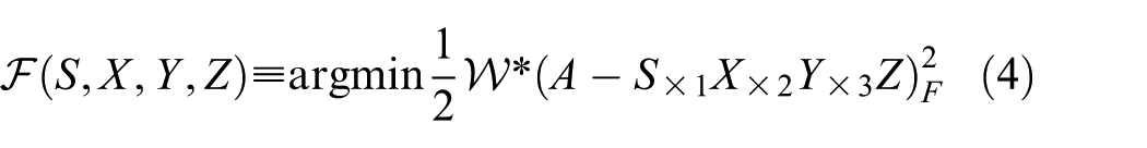
where

It should be noted that the function

When setting

Given the partial derivatives of the regularized cost function

Segment travel time estimation
This section presents the travel speed and travel time calculation; the estimator is driven by reconstructed transit trajectory and produces accurate estimations

Trajectories in space and time based on the inferred transit AVL data.
In Figure 5, the local time-mean speed

Instantaneous space-mean speed

Then we can estimate the probe travel time using the distance of the road section D dividing the instantaneous space-mean speed

where
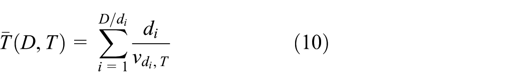
where
Case study
In this section, a case study is illustrated for estimating the transit travel speed and travel time on the consecutive route segments on 23 Ave. in Edmonton, Canada. As shown in Figure 6, the test route is on a 3.2-km stretch of a main urban corridor, which includes seven bus stops and seven intersections (five signal intersections and two non-signal intersections) from Tegler Gate bus stop to 111 Street. The speed limit is 60 km/h. We set up eight path points in the bus stops to separate the route into seven segments, and thus the delay of transit would be eliminated to some extent when we evaluate the travel speed on each separated segment.

Transit route on 23 Ave. with intersections and bus stops identified.
The transit AVL system broadcasts records containing the location (latitude, longitude), timestamp, and vehicle ID once every 30 s on average. In this case, totally 5364 observations generated by 336 trips on 23 Ave., in Edmonton from 4 to 11 July 2016, are used as the samples. The total length of the trajectories is over 1407 km.
We map-matched the collected transit probe raw data into the scheduled route and estimated the bus travel information in the corresponding route segments and time slots, based on which we created two tensor models

where M is the number of non-zero entries and N means the total number of entries in the tensor
where
Results and discussion
In this section, the performance of the tensor-based method for inferring the missed probe travel time information in specific time slots and route segments is assessed. Based on the reconstructed trajectories, the local time-mean travel speed and the average travel time on each route segment over time of day were supposed to be estimated and evaluated.
The results of the inferred probe travel time information are investigated, as shown in Figure 7. The tensors

(a) Reconstructed travel speed field, (b) statistics of non-zero entries in tensor, and (c) performance of trajectory reconstruction.
In addition, the performance of the tensor-based method is evaluated using the current probe sample set and both the current and historical sample sets, and the result is shown in Figure 7(c). It seems that tensor-based decomposition usually performs well on inferring missed values (i.e. transit travel speed over road segments in each time slot), but fails to converge as the percentage of missing entries increases. For example, during the period 14:30–15:00, each entry in
Based on the reconstructed travel information, the local time-mean travel speed and the average travel time on each segment over time of day were estimated and evaluated, as shown in Figure 8.
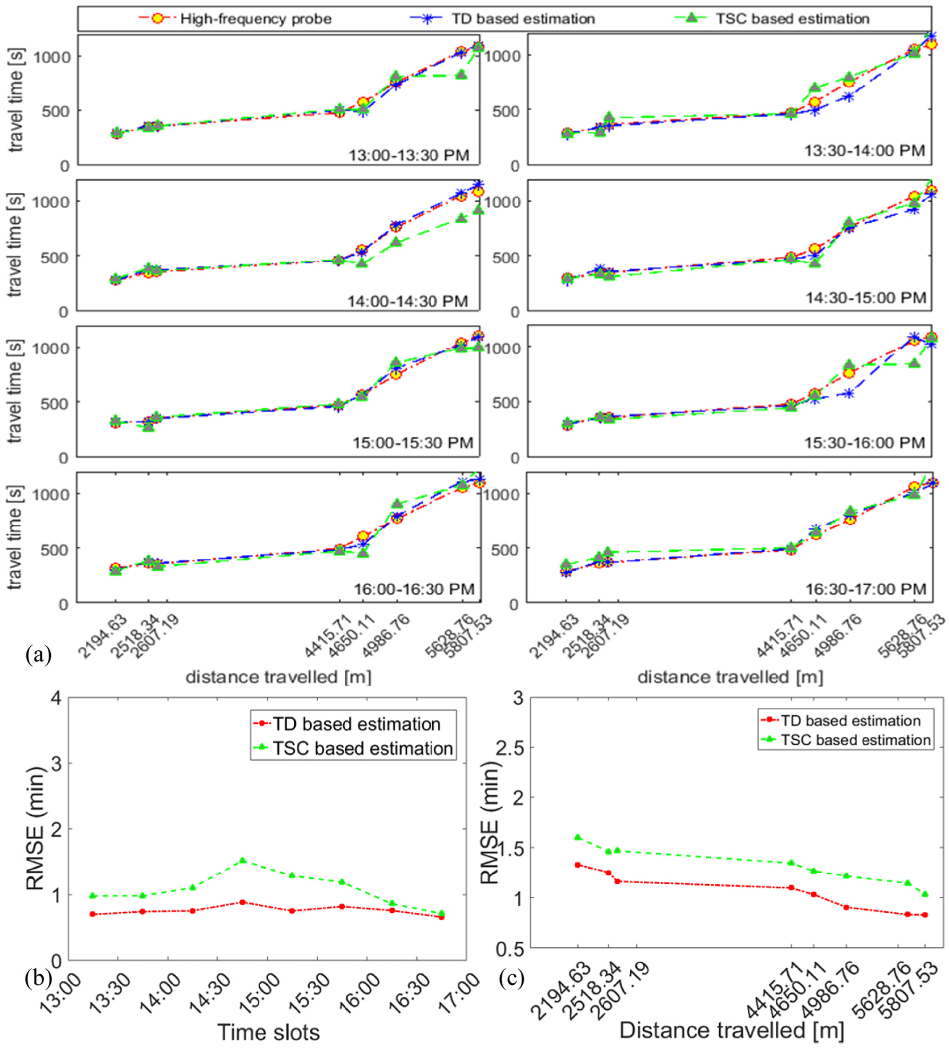
(a) Travel time estimation results, (b) performance of travel time estimation changing over time of day, and (c) performance of travel time estimation changing over route segments.
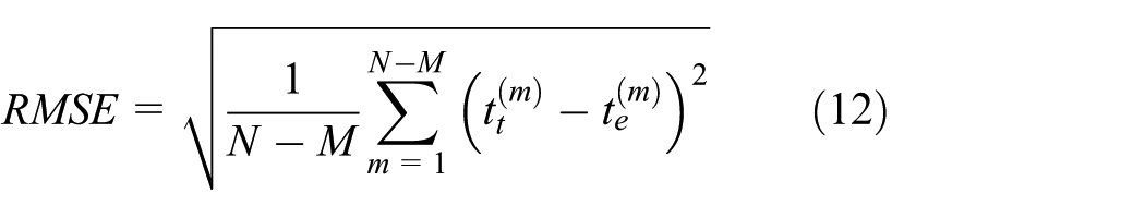
Based on the estimated transit local time-mean travel speed changing over time of day, we estimated the transit travel time passing different segments in Figure 8(a). We compared the performance of travel time estimation based on the TD method with the trajectory-based simple concatenation (TSC) method as shown in Figure 8(b) and (c). The TSC method examines the road travel time information on each segment using mainly the previously passed probe trajectories in the recent short-term period. 19 If the measurement of probe records on a certain segment is missed or very sparse, it is supposed to use the previous estimated travel time instead and accumulate the estimated results on each segment as the summation of travel times along the traversed path.
Figure 8(b) presents the performance of our method and TSC changing over time of day. The TSC-based estimation on road segments deviates the true travel time in free traffic hours, around 14:30–16:00, for example, the RMSE of TSC-based estimation is 1.55 min during 14:30–15:00. When it is in peak traffic hours, that is, 16:00–17:00, the error of TSC-based estimation decreases and comes close to TD-based estimation. This result illustrates that the TSC-based method fails to provide accurate estimation if the size of the probe sample cannot meet the minimum requirement. When there are not enough transit buses traveling on road segments, for example, during 14:30–16:00, the error of TSC is higher than that in the other time slots. However, the RMSE of estimation using our method increases only slightly during free traffic hours. This demonstrates the effectiveness of inferring the unobserved trajectories.
Figure 8(c) shows the results of the average travel time estimation on each segment along the path. The errors of using TSC and our proposed method for estimation decreased as the traveled distance is increased. As the length increases, the more sample size would be involved than in the shorter subpath. Especially, the travel time of a separated segment is significantly impacted by intersections and bus stops. In such condition, it turns out to be difficult to estimate this segment travel time in dynamic traffic situations.
Conclusion
In this article, we have shown how to effectively make use of sparse bus probe data in measuring the transit route travel speed and travel time in different temporal and spatial blocks. These data provide a good coverage of the current and historical contexts learned from bus trajectories and map data. We also have shown in our use of the 3D tensor model that a great deal of sparse uncounted transit route travel time can be derived from the existing data. Thereafter, a general prescription of estimation was proposed to evaluate the transit route efficiency at any point for a bus traveling on a known path. The results of the extensive experiments demonstrate the advantages of our method.
In addition, in the future, transit probe may prove a feasible data source and is more amenable to arterial travel time calculations. The transit probe data increase the probe sample size along the corridor compared to the use of only general probe, which in turn make arterial travel time calculation more accurate. In the future studies, considering the fact that transit vehicles and general vehicles have different running behaviors, that is, delay and dwelling time at the bus stop, a bias has to be investigated between transit travel time and arterial travel time. Also, the travel times on different segments are assumed to be independent conditional on the state of the system, which lead to incorrect estimates of the travel time variability on certain routes. Therefore, the proposed method should be improved by incorporating more factors related to transit reliability, that is, traffic congestion and weather conditions.
Footnotes
Acknowledgements
The authors gratefully thank the City of Edmonton for providing the transit GPS records and road network data for the case study.
Handling Editor: Zhixiong Li
Declaration of conflicting interests
The author(s) declared no potential conflicts of interest with respect to the research, authorship, and/or publication of this article.
Funding
The author(s) disclosed receipt of the following financial support for the research, authorship, and/or publication of this article: This work was partially supported by the Jiangxi Provincial Fund for Visiting Scholar Development Plan (Grant No. 2016109), Jiangxi Provincial Department of Education Science Research Fund Project (Grant No. GJJ170420), and ECJTU “TIANYOU Talent” Development Program (Grant No. 201709).