Sage Journals: Discover world-class research

Abstract

This study proposes a novel active screw-drive in-pipe robot that can adapt the circular-type and square-type pipe structure. The pipe robot is composed of four driving units and a wall-pressing suspension mechanism. Each driving unit contains a motor, a transmission train, and an electromagnetic brake, which is for switching the motion transmission route. DC motors drive the helical wheels, and the incline angle of the helical wheels can be adjusted by using the electromagnetic brake. The wheels of the driving unit exhibit rolling and steering motion. Thus, the robot is capable of translation movements, rotation movements, and screw motions with respect to the axis of the pipe according to the different positions of the helical wheels. The robot can avoid obstacles by using the rotation and screw modes. Moreover, the wall-pressing mechanism is analyzed and modified, and a criteria for entering a reduction pipe reducer are derived for the double scissor-like suspension mechanism. We also analyze the robot motion in curved pipes in two typical postures. The simulation experiments reveal the relationship between the translation and rotation motion of the robot and indicates that the steering angle of the wheels can be regarded as a regulator to adjust the movement speed of the robot aside from tuning the posture of the robot. Elbow experiments are conducted to verify the effectiveness of the motion strategy. The robot can be adapted for both circular and square tube pipes without any change in its structure due to the special configuration.

Keywords

Pipe robot active screw drive mechanism design slider-crank mechanism

Introduction

Pipes are widely used to transport many types of fluid in modern societies, and they provide convenience for daily life and mass industrial production. Aging pipes are prone to internal corrosion, leakages, and cracks due to chemical elements or high pressures. Pipes must be checked periodically to prolong their lifecycle, reduce maintenance expenses, and prevent severe accidents.

However, several pipelines are public facilities and buried underneath the ground. They have limited space and are very difficult to access. To send inspection tools into pipes, researchers have developed many kinds of robots that can enter the confined space of pipelines. The moving principle of pipe robots can be divided in two main types, namely, passive and active. The most common passive-type is PIG, which is driven by the pressure of the fluid in the pipe.

Hu and Appleton¹ developed a PIG type with a bush-traveling mechanism in pipes. Nguyen et al.² developed a PIG pipe robot that can pass through curved section pipelines for natural gas.³ Meanwhile, active-type robot are equipped with motor/actuator to generate propulsion force in the pipe. The most typical active-type pipe robot is the wheel-type robot^4–8 and crawler-type robot.⁹ The wall-pressing mechanism is a necessity to generate traction force to pull itself and increase payload, and this mechanism can be divided into passive⁴ and active types.¹⁰ The passive wall-pressing mechanism is usually supported by springs and other elastic elements to press the driving wheel/tracks or legs on the inner surface of the pipe.^4,5 The active-type wall-pressing mechanism uses the motor to hold the entire configuration of the robot. Using these mechanisms, pipe robots can move rapidly and possess a high payload capacity. Articulate pipe robots have highly complex structures and control algorithms to coordinate the entire body motion,^11–15 but they are flexible in principle. Mini pipe robots are also developed to work inside the human body, and these robots can travel in vessels.¹⁶

For curved pipes, several wheeled robots can pass through the pipe elbow due to their delicate design, and classic structures have been formed to pass through the T branch.^4,9 Adaption of robots in pipe environments still possess limitations. For example, these robots can only move in circular-shape pipes, and can seldom move in square-shape pipes without changing the structure. Therefore, the adaptability of the robot’s moving mechanism can still be improved.

Pipelines in daily life and industrial applications have circular and square tube shapes that are in accordance with the cross-sectional shape, as shown in Figure 1. Circular tube–shape pipes are commonly used due to their symmetry, and most robots can move in this enviroment.^4–9 Square tube–shape pipe can be seen in air conditioning circulation loops and other unsealed gas transportation.

Figure 1.

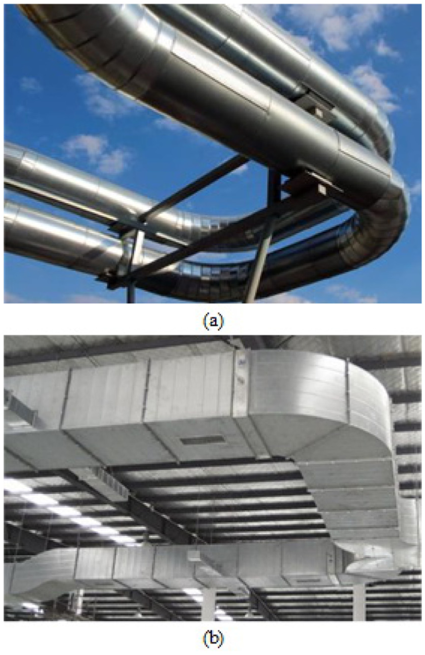
(a) Circular and (b) square tube pipelines.

These pipes have different maintenance requirements. Pipe robots can only adopt a specific pipe shape and seldom can adopt circular and square tube shapes simultaneously. From the traditional view, almost every kind of pipeline inspection requires one custom-designed robot. A pipe robot with versatility can reduce the deployment cost for the service company, and it is an important feature in daily inspection tasks because it not only expands the application scenarios but also increases the execution efficiency of the inspection system. Thus, developing versatile robots or robots with adaptability would benefit users and manufacturers.

In this study, we aim to design a robot that can move not only in circular tube pipes but also in the square tube pipes to extend the adaptability of the robot. The difficulties involved in designing such a robot include the steering ability, obstacle avoidance capability, and adaptability to pipe shape changes. Many wheeled and caterpillar pipe robots have good steering capability but can seldom moves in circular and square pipes simultaneously.

We employ the screw-drive principle to design a robot that can move in circular and square pipes.⁶ This principle is explained in Figure 2. The robot is composed of a rotator, a stator, and rollers that are hinged on the rotator at an incline angle. The rotator rotates around the center axis of the pipe, and the whole robot moves along the center axis. Given that the roller wheels are passive, they have a spiral motion with respect to the center axis of the pipe.

Figure 2.

Screw-drive principle of the pipe robot.

We set the wheels at an incline angle with respect to the axis of the pipe, and the motors drive the wheels directly in this study. As a result, the robot can also exhibit the spiral motion along the pipe axis. By adjusting the incline angle of the wheels, we can control the robots angular and translational velocities to adapt to the shape of the pipes. We also design a suspension mechanism that pushes all the wheels against the inner wall of the pipe, and this can guarantee movement and traction capability in the pipe.

The rest of the article is organized as follows. Section “Design of the active screw-drive robot” introduces the design of the robot, including the driving unit, the steering, and the wall-pressing mechanism. Section “Analysis of motion in the pipe” provides an analysis of the robot in curved pipes by using two typical postures and a motion strategy. Section “Simulation experiments” presents the simulation results and velocity relations of the robot in straight pipes and elbows.

Design of the active screw-drive robot

We design an active screw-drive robot for use in circular and square tube pipes (Figure 3). The robot is composed of three main modules, four driving units, a steering mechanism, and a wall-pressing mechanism.

Figure 3.

Active screw-drive in-pipe robot.

The wheels in the diving unit are different from previous passive helical wheels. The wheels in this design are driven by motors via a gear train, and the motions of the motors are transmitted to the motion of the active helical wheels. The robot has four driving units, which are located on the four corners of the robot and form a rectangle shape in the axial direction of the pipe. In the cross-section of the robot, a slim rectangle shape is formed due to the necessity of having a mechanical structure.

The function of the wall-pressing mechanism is to apply positive force to the active helical wheels so that the wheels can have firm contact with the inner surface of the wall. The wall-pressing mechanism is located in the middle of the robot and forms a skeleton of the robot by using a scissor-like mechanism by which the active helical wheels can extend and contract according to the change in diameters. The springs are placed between the central axis and the sliders to generate pressing force for the wheels.

The steering mechanism is coupled with the driving mechanism, and we use an electromagnetic brake to switch the motion transmission route of the motor. Hence, by controlling the electromagnetic brake, the active helical wheel can change the incline angle with respect to the axis of the pipe. The active helical wheel has 2 degrees of freedom (DOF); One DOF is the rolling motion of the wheel itself, and the other DOF is the steering motion of the wheel. By changing the direction of the helical wheel, we can change the posture and motion mode of the robot. Then, the robot can adapt to circular and square tube pipes.

By using the power switch structure, we reduce the number of motors to one for each unit, thus reducing the entire system cost because the electromagnet is cheaper than the servo motor. The structure is also reduced to two parts, namely a driving unit for driving and steering the wheel and a wall-pressing mechanism for generating adhesion force.

As shown in Figure 3, the four driving units and scissor-like mechanism are designed and placed symmetrically. The robot thus has bi-directional drive capability and can easily balance from disturbance. Furthermore, the driving unit is designed as a module. It is, therefore, easy to install and replace in case it does not work.

Driving unit

The driving units are used to transmit power from the motor to the helical wheels. For the convenience, the upper/lower half of the two units shares the same motor base. A driving unit has a pair of spur gears, two pairs of bevel gears, an electromagnetic brake, and a DC motor, as shown in Figure 4. The gear transmission has high accuracy and high payload, and the spur gear can amplify the output torque of the motor and reduce unexpected impact to the motor. For control reliability, all motion transmission or reversion is realized by the gear.

Figure 4.

Structure of the driving unit.

The principle of the driving unit is shown in Figure 5. The motion of the DC motor is adjusted to $9 0^{\circ}$ with respect to the axis of the motor by bevel gears 1 and 2, and the speed is decreased by spur gears 3 and 4. The axis of spur gear 3 passes though the center hole of the electromagnet brake and is connected with bevel gear 5. Bevel gear 6 is fixed on the axis of the helical wheel and can drive two helical wheels located on the side of the wheel carrier. The motor and electromagnet brake are fixed on the base. The axes of the spur gears 3 and 4 are hinged on the base. The brake ring and the electromagnet brake’s main body have teeth, which can engage each other due to the magnetic force. They can also stick together. The brake ring and wheel carrier form a sliding joint. Thus, the brake ring can slide on the wheel carrier when the magnetic force disappears.

Figure 5.

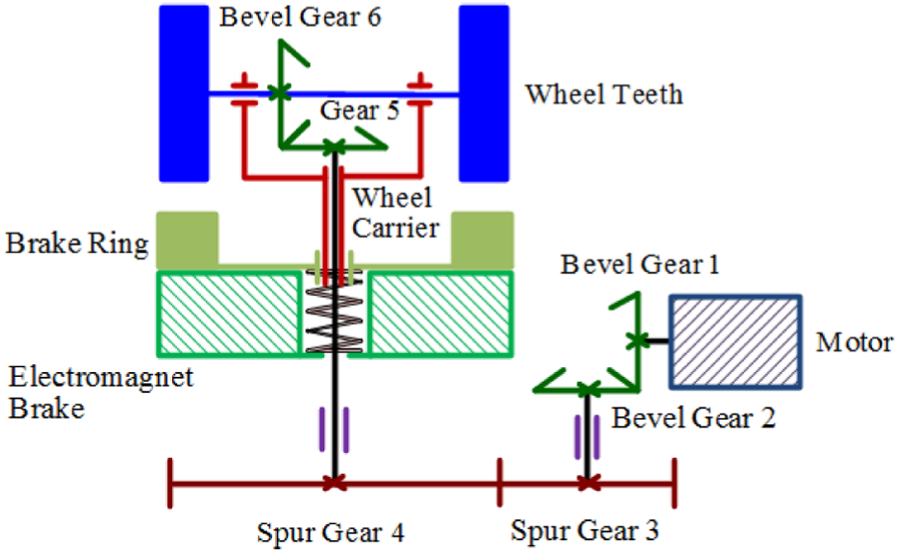
Driving transmission route of the drive mechanism.

The flat configuration of the driving unit is designed to save space along the radial direction, and its extension and concentration ratio can affect the adaptability to diameter change.

As indicated in Figure 6, we fix an electromagnet brake on the base of the driving unit, which means the brake cannot move with respect to the motor. A permanent magnet and a coil winding are located inside the electromagnet brake. The brake ring with teeth is attached to the surface of the main body of the electromagnet brake due to the magnet force of the permanent magnet. A spring is placed between the brake ring and the main body of the electromagnet brake to resist the magnetic force.

Figure 6.

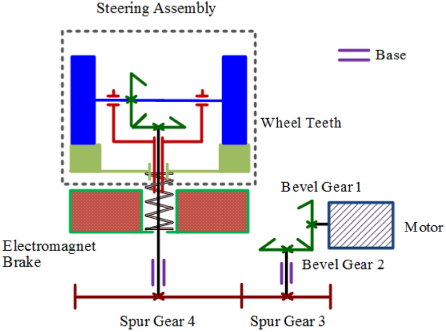
Steering transmission route of the drive mechanism.

The steering motion of the wheel requires the coordination of the brake, spring, wheel carrier, bevel gears 5 and 6. The permanent magnet–type brake in Figures 6 and 7 has a hollow hole structure that allows the axis of spur gear 4 to pass through concentrically. A spring, which sheaths the axis of spur gear 4, is set between the brake ring and the main body of the brake.

When the coil winding in the brake is electrified, the magnetic field from the coil is opposite to that of the permanent magnet. The magnet force, which attaches the braking ring to the main body, is weakened. As a result, the brake ring is disengaged from the main body of the brake and is extended by the recovery force of the spring.

As indicated in Figure 7, each helical wheel is attached to a gear pinion concentrically, and a segment of a rack is fixed under each pinion. Each brake ring has two racks and can engage with the pinion when the spring pushes the brake ring along the axis of spur gear 4.

Figure 7.

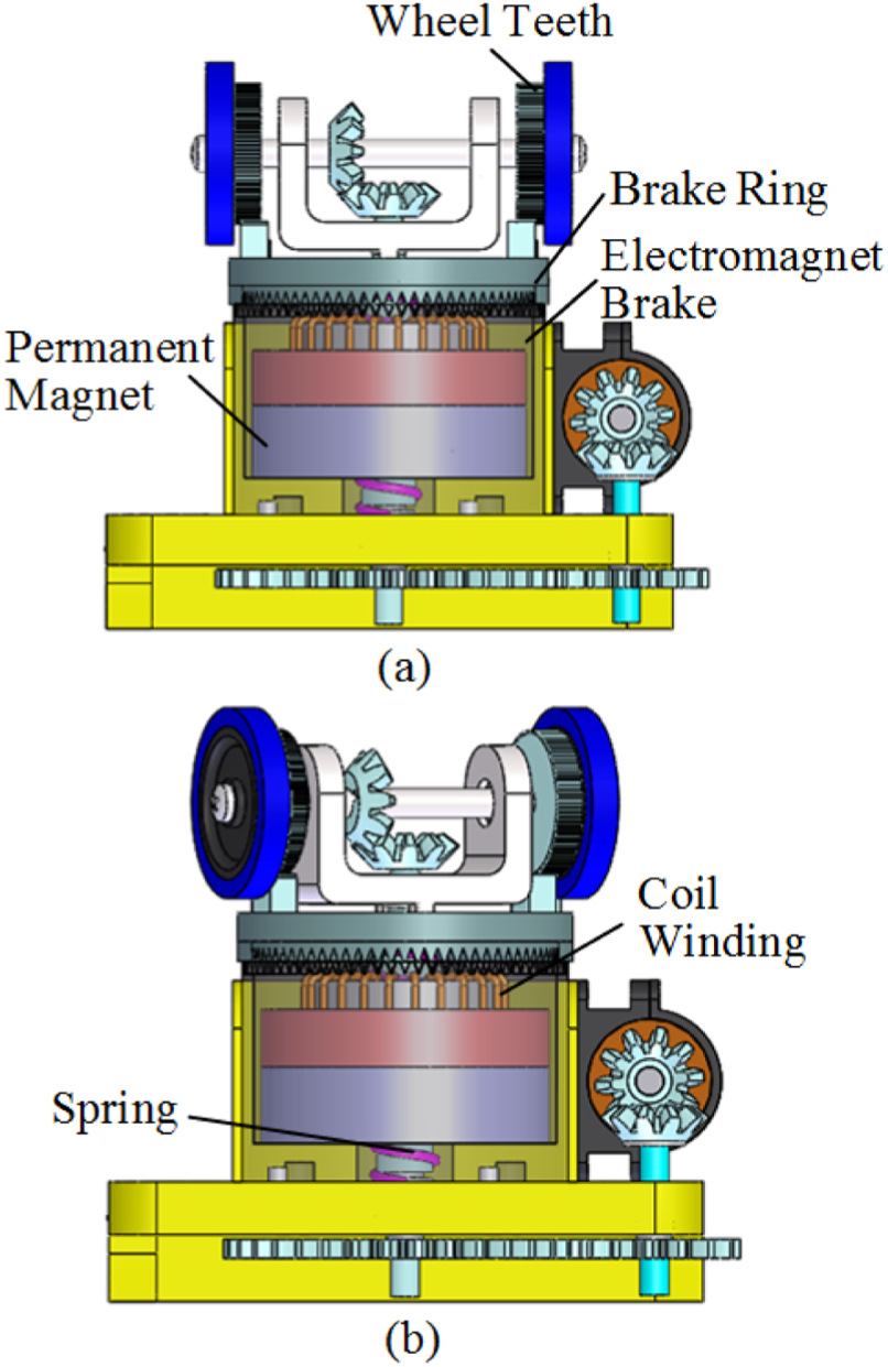
Movement of steering motion.

For the steering motion, the electromagnet brake is powered on, and the magnetic field of the coil winding counteracts that of the permanent magnet. The spring pushes the brake ring out, and the brake ring slides toward the teeth wheel. Then, the brake ring and teeth wheel engage together. At this moment, the brake ring, wheel carrier, bevel gears 5 and 6, teeth wheel, and helical wheel kinematically stick together, as shown by the red square with a dash line (steering assembly) in Figures 6 and 7(a).

Thus, when the brake ring engages with the pinion, the motor drives bevel gears 1 and 2 and spur gears 3 and 4. The whole steering assembly rotates together with spur gear 4. The angle of the helical wheel on the driving unit is adjusted, as indicated in Figure 7(b).

By using a motor and a brake, the driving unit has two working statuses.

Driving status: when the brake is powered off, the motion is transmitted from the motor to bevel gear 6, and the helical wheel rotates to drive the robot forward and backward.

Steering status: when the brake is powered on, the motion of the motor will be transmitted to spur gear 4, and the motor turns the entire steering assembly to rotate with respect to the axis of spur gear 4. This status adjusts the posture of the robot.

The reason we use a permanent magnet–type brake is that the brake does not consume extra energy to maintain the status. In principle, both permanent and non-permanent magnet types are eligible for the above mechanism.

Let $i_{i, j}$ be the transmission ratio from i to j and $z_{i}$ be the tooth of gear i. The ratio from the motor to the helical wheel $i_{1, 6}$ is as follows

i_{1, 6} = \frac{z_{6} z_{4} z_{2}}{z_{5} z_{3} z_{1}}

(1)

The ratio from motor to the steering motion $i_{1, 4}$ is

i_{1, 4} = \frac{z_{4} z_{2}}{z_{3} z_{1}}

(2)

Then, we can obtain the scalar relationship of the motion of the helical wheel and motor angular velocity $ω_{m}$ . Let $ω_{w}$ be the angular velocity of the helical wheel and $ω_{s}$ be the angular velocity of the steering motion. We know that

ω_{w} = \frac{ω_{m}}{i_{1, 6}}

(3)

ω_{s} = \frac{ω_{m}}{i_{1, 4}}

(4)

The speed relationships of the driving unit are derived. Suppose that the payload of the robot is 30 N, then each side of the robot bears 15 N. Considering that the driving wheel of each side may slip, the payload for each driving wheel is 15 N. The rated velocity of the robot is 0.125 m/s, and the power of the DC motor is 1.875 W. We use three pairs of gear trains and a gearbox for the motor, and the efficiency of the entire transmission is approximately 0.5–0.6. The power of the driving motor should be between 3.125 and 3.750 W. Therefore, a Maxon RE 16 motor with 3.2 W rated power is selected, considering that we have already introduced the traction redundancy. The rated speed of the motor is 5990 r/min, and the frequency of the motor is 99.83 versus that of the driving wheel, which is 2. Thus, the total transmission from the motor to the driving wheel is 49.9. We select four bevel gears to change the direction of the motion and a gearbox GP16 (item No. 416628) for the motor with a ratio of 1/29. The transmission ratio of the spur gear is 1/1.72. The teeth are as follows: $z_{1} = z_{2} = z_{5} = z_{6} = 20$ , $z_{3} = 17$ , and $z_{4} = 29$ .

Wall-pressing mechanism

The classic wall-pressing mechanism is the slider-crank mechanism, and this wall-pressing mechanism is usually composed of two slider cranks.⁴ The two of the slider cranks can work independently, but a slight difference is observed when we connect them together. Figure 8 shows the problem. A_i, B_i, P_i, and O_i denote the hinge of two parts including bars and sliders. When $A_{1}$ and $A_{2}$ are connected, kinematically speaking, $A_{1} A_{2}$ can only move parallel to $O_{1} O_{2}$ . We need to modify one of the kinematic constrain. For example, we want $A_{1} A_{2}$ to have an extra degree of freedom and then rotation must be done with respect to any convex.

Figure 8.

Double slider-crank mechanism.

A feasible approach is to make the inner hole of the slider larger than the diameter of the axis, as shown in Figure 8(b). In this case, the entire mechanism is converted into two mechanisms. $O_{2} A_{2} P_{2} B_{2}$ is a slider-crank mechanism and $A_{2} A_{1} P_{1} O_{1}$ is a four-bar mechanism. The contact between the $B_{1}$ slider and the axis can be regarded as a position limit. This solution can address the current problem, as indicated in Figure 9.

Figure 9.

Modified slider-crank mechanism.

Figure 9(a) shows the result of modifying the contact condition of the slider and axis, $A_{1} A_{2}$ obtains an extra degree of freedom.

When we duplicate a mirror structure with respect to the axis, the modified slider can still coordinate the motion of the linkage, but the upper and lower parts do not have an expected symmetric motion, as shown in Figure 9(b). The solution still has a kinematic defect when it is considered as the skeleton of the robot.

Several pipe robots have a spatial symmetric configuration. Thus, the kinematic defect exerts little effect on motion stability. The robot we propose has a flat surface structure in the cross-sectional direction, and it needs a kinematically feasible wall-pressing mechanism to guarantee symmetry. Based on the above mechanism, we introduce a sliding joint between $A_{1}$ and $A_{2}$ to coordinate the motion conflict in Figure 8. The configuration of the mechanism in Figure 9 shows the maximum incline position, where $∥ O_{1} P_{1} ∥ = L_{1}$ , $∥ A_{1} B_{1} ∥ = ∥ A_{2} B_{2} ∥ = L_{2}$ , $∥ O_{1} O_{2} ∥ = L_{0}$ . The incline angle of $θ_{1}$ is

\tan θ_{1} = \frac{\sqrt{L_{2}^{2} - ∥ O_{2} B_{2} ∥^{2}} - \sqrt{L_{2}^{2} - ∥ O_{1} B_{1} ∥^{2}}}{L_{0}}

(5)

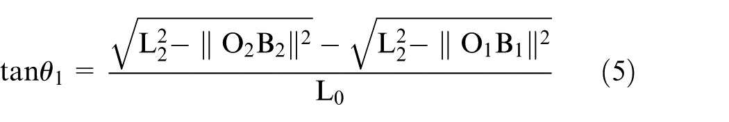
By using this equation, we can calculate the maximum extension and the minimum contraction diameters of the robot. The maximum incline angle of $A_{1} A_{2}$ is

lim_{∥ O_{2} B_{2} ∥ \to 0} \tan θ_{1} = 1

(6)

If the physical structural width of $B_{2} O_{2}$ is reduced from $0.2 L_{2}$ to $0.1 L_{2}$ under the condition of $L_{0} = L_{2}$ , the incline angle of $A_{1} A_{2}$ increases rapidly, as indicated in Figure 10. The maximum incline angle of this double slider-crank mechanism is $45^{\circ}$ . In this case, $∥ O_{2} B_{2} ∥ + ∥ O_{1} B_{1} ∥ = L_{2}$ , which is an additional constraint. In the case of $L_{0} = 2 L_{2}$ and $L_{0} = 3 L_{2}$ , the length of $∥ O_{1} O_{2} ∥$ is bigger than $∥ O_{2} B_{2} ∥ + ∥ O_{1} B_{1} ∥$ . Therefore, the maximum incline angle decreases accordingly. For the practical usage, the length ratio is should be below 0.2, and the length of $∥ O_{1} O_{2} ∥$ should be small to maintain a wide range of adoption.

Figure 10.

Proposed wall-pressing mechanism for the robot.

We also need to check the concentric reduction adaptor and determine if the length of the adaptor satisfies the following condition in the entire pipeline structure

Lengt h_{adaptor} < \frac{Diamete r_{large} - Diamete r_{small}}{2}

(7)

Then, we can use the double slider-crank mechanism as the wall-pressing mechanism to ensure the accessibility of the small pipes.

The wall-pressing mechanism of the robot uses the configuration in Figure 11, which ensures the motion relationship rigorously and is easy to calculate during mechanism analysis if we select the $L_{2} = 2 L_{1}$ . The two sliders, $B_{1}$ and $B_{2}$ , are pressed by two springs, and the driving units are fixed on the supporting plate, which is $A_{1} A_{2}$ .

Figure 11.

Relation between length ratio and incline angle of $A_{1} A_{2}$ .

By using the kinematic relation, we can approximate the spring force based on the following relation

\frac{F_{n_{w}} \cos θ_{p}}{F_{sp} - F_{n_{w}} \sin θ_{p}} = \frac{1}{\sqrt{{‖ \frac{A_{1} B_{1}}{O_{1} A_{1}} ‖}^{2} - 1}}

(8)

where $F_{n_{w}}$ denotes the normal force of the wheel and surface contact, $F_{sp}$ denotes the force of the spring, and $θ_{p}$ is the contraction of the pipe diameter. In a straight pipe, $θ_{p}$ is $0 \circ$ . We set the ratio of $A_{1} B_{1} / O_{1} A_{1}$ from 0 to 1 to determine if $F_{sp}$ provides sufficient reaction force during movement.

Motion modes

The proposed robot has three motion modes in the pipe: straight, rotation, and screw.

Straight motion mode: the incline angle of the helical wheel is $90 \circ$ with respect to the cross-section of the pipe, which means the axis of the helical wheel is perpendicular to the axis of the pipe. The robot moves forward and backward and only has a translational motion.

Rotation motion mode: the incline angle of the helical wheel is $0 \circ$ with respect to the cross-section of the pipe. The robot rotates around the axis of the pipe and only has rotation motion.

Screw motion mode: the incline angle of the helical wheel lays between $0 \circ$ and $90 \circ$ with respect to the cross-section of the pipe. The robot has translational and rotational motions.

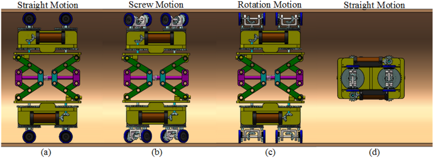
These motion modes are helpful. For example, the robot adjusts its posture to avoid collision or pass through a complicated structure of the pipe. Figure 12 shows a typical posture change. Figure 12(a) shows the robot moving in the pipe in the straight motion mode. Then, the helical wheels change to $0 \circ$ and begin to rotate around the pipe axis, as shown in Figure 12(c). When the robot turns by one quarter, the helical wheels turn back to $90 \circ$ again and keep on moving, as indicated in Figure 12(d). By changing the motion mode, the robot adjusts its posture, which is beneficial to obstacle avoidance. During the transition from straight motion to rotational motion, screw motion occurs, as presented in Figure 12(b). This is also important for the robot because pure rotation mode is seldom used; most of time, the robot uses screw motion to tune its posture.

Figure 12.

Motion modes of the pipe robot.

Analysis of motion in the pipe

By using the three motion modes, the robot acquires many motion control strategies to pass typical pipes. The elbow is a common pipe structure. Therefore, we need to perform a motion analysis of the robot. The robot has two typical postures when it passes an elbow. Figure 13(a) shows the robot moving in the cross-section of the elbow (posture A), and Figure 13(b) shows the robot moving in the vertical section of the elbow (posture B).

Figure 13.

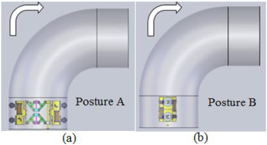
Two postures to pass the elbow.

Posture A in the elbow

The motions of the wheels differ. Three stages occur when the robot uses posture A. First, the two fore wheels enter the curve. Second, the entire robot enters the curve. Finally, the front wheels enter into the straight pipe while the rear wheels stay in the curve. The first stage is shown in Figure 14.

Figure 14.

First motion stage in the elbow using posture A.

The pipe diameter is D, and the radius of the curvature is R. $v_{wi}$ represents the wheel velocity of the first stage, $ω_{i}$ represents the $i th$ wheel, and $r_{w}$ is the diameter of the wheel. In the first stage, the fore wheels enter the curvature and the rear wheels are still in the straight section. The angular velocity of the robot is

ω_{r} = \frac{ω_{1} r_{w}}{R + 0.5 D - r_{w}} = \frac{ω_{2} r_{w}}{R - 0.5 D + r_{w}}

(9)

O is the instantaneous center of motion. The coordinate of wheel 2 $(x_{2}, y_{2})$ is $((R + r_{w}) \sin δ_{1}, (R + r_{w}) \cos δ_{1})$ . $δ_{1}$ is the span angle of wheel 2. $(x_{4}, y_{4})$ is the coordinate of wheel 4, and $y_{4} = (R + 0.5 D - r_{w})$ . We can obtain $x_{4}$ by using the following constrains

(x_{4} - x_{2})^{2} + (y_{4} - y_{2})^{2} = {l_{r}}^{2}

(10)

Similarly, $x_{3}$ can be derived by using $x_{1}$ , $y_{1}$ , and $y_{3}$ . Then, the length of $W_{4} O$ , $∥ W_{4} O ∥$ , can obtained with $(x_{4}, y_{4})$ . The same applies to $∥ W_{3} O ∥$ . Thus, the rear wheels have two options for passing: one is passive mode and the other is active mode.

For passive mode, the rear wheels follow the entire body motion and do not contribute traction force. Thus, the velocity of wheels 3 and 4 is

v_{wi} = ω_{r} ∥ W_{i} O ∥

(11)

Given that the rear wheels are passive, the robot can easily enter the curvature of the elbow. This mode is preferred when the payload is not high. The other option is that the rear wheels contribute to traction force, and the angular velocity of the wheel needs to satisfy the following

ω_{wi} r_{w} \leq ω_{r} ∥ W_{i} O ∥ \cos δ_{i}

(12)

This condition means that the velocity of the rear wheels does not push the fore wheels to slip, and the normal element of driving velocity $ω_{wi} r_{w}$ can induce the contraction and extension of the wall-pressing mechanism.

In the second stage (Figure 15), when the rear wheels enter into the curvature, the angular velocity of the robot is

ω_{r} = \frac{ω_{w 1} r_{w}}{R + 0.5 D - r_{w}} = \frac{ω_{w 2} r_{w}}{R - 0.5 D + r_{w}}

(13)

Figure 15.

Second motion stage by using posture A.

The velocity ratio of the wheels on the outer ring versus that of the inner ring is

r_{curvature} = \frac{ω_{w 1}}{ω_{w 2}} = \frac{R + 0.5 D - r_{w}}{R - 0.5 D + r_{w}}

(14)

As long as the velocity ratio of the outer wheels versus the inner wheels is stable, the robot will move smoothly in the elbow. According to the above equation, we can calculate the velocity of the four wheels. The condition in the third stage is similar to that in the first stage. The fore wheels recover to an equal speed, and the rear wheels become passive.

Posture B in the elbow

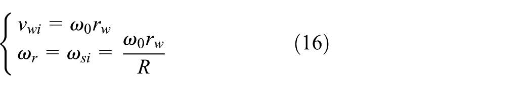
The illustration in Figure 16 shows the robot passing the elbow in the vertical section of the elbow (Posture B). Three stages are also observed. In the first stage, the fore wheels enter the curvature, and the velocity of the fore and rear wheels can be described by the following equations

{\begin{matrix} v_{w 1} = ω_{0} r_{w} \\ ω_{r} = ω_{s 1} = \frac{ω_{0} r_{w}}{R} \\ δ_{1} = \int_{0}^{t} ω_{r} (t) dt \\ v_{w 3} = v_{w 1} \cos δ_{1} \end{matrix}

(15)

where $ω_{0}$ and $ω_{si}$ represent the wheel and steering angular velocities, respectively, and $δ_{1}$ represents the sector angle of the fore wheels. The last expression guarantees the velocity coherence for the rear wheels in the straight section.

Option 1: When we set the fore wheels as the active wheels, the angular velocity of the robot $ω_{r}$ and the steering angle $ω_{s 1}$ are easy to determine. Then, the velocities of the rear wheels are determined under the condition of velocity coherence.

Option 2: When the rear wheels are active wheels, $ω_{r}$ needs to be acquired first in order to obtain the velocity of the fore wheels. After solving a differential equation, the value of $ω_{r}$ is derived, and $v_{w 1}$ and $ω_{s 1}$ are determined.

Figure 16.

Motion analysis by using posture B.

In Option 1, all of the values of the system can be derived easily, but the rear wheels encounter a velocity inconsistency at the start of the second stage in the elbow. Option 2 eliminates this velocity inconsistency between the first and second stages, but we need to solve the differential equation first, which causes inconvenience in practical use.

For the second motion stage, the fore and rear wheels are in the curve section; the velocity of the robot can be described as

{\begin{matrix} v_{wi} = ω_{0} r_{w} \\ ω_{r} = ω_{si} = \frac{ω_{0} r_{w}}{R} \end{matrix}

(16)

The motion of the four wheels falls under the same condition until the robot runs out of the curve section. For the third motion stage, the motion of equation is the same, and it is a mirror process of the first motion stage. Notably, the strategy of posture B in the elbow is also suitable of T-shape pipes because the vertical sections of the elbow and T-shape pipes are highly similar and even large in the center zone. As long as the robot can pass the elbow in posture B, the robot can also pass a T-shape pipe with the same diameter.

When the robot moves in the curved pipe, the length and width of the robot must satisfy geometric conditions.¹⁷ We found that the maximum length of the robot is related to the relative shape configurations, as indicated in Figure 17. We investigated four typical conditions, let $R$ be the radius of the elbow curvature, $D$ is the diameter of the pipe and $δ_{e}$ be the span angle of the curve section. Figure 17(a) and (b) shows that span angle $δ_{e}$ is larger than $90 \circ$ , but the robot (red rectangle) can have two positions in the elbow. One condition is that the robot falls into the curve sector completely, as shown in Figure 17(b), and the other is that the robot body can still stay in the straight part. This phenomenon also occurs in the condition of span angle $δ_{e}$ being smaller than $90 \circ$ . Thus, a condition dominates these configurations. Suppose that the robot no longer has width d, and it degrades into a line $l_{r}$ . Then, the critical condition arise when

δ_{e 0} = \arccos \frac{R - 0.5 D}{R + 0.5 D}

(17)

When the span angle $δ_{e}$ of the elbow is larger than $δ_{e 0}$ , the robot body completely falls into the curve section. When $δ_{e}$ is smaller than $δ_{e 0}$ , the robot body can be maximally extended to the straight part of the pipe regardless of R and D. Equation (17) becomes the first step to calculate the span angle of the elbow with this critical value $δ_{e 0}$ and identifies the relative shape relationship between the robot and pipe.

Figure 17.

Relative configurations of the robot and pipe geometric shape.

Figure 17(a) shows that the whole length $l_{r}$ is double the sum of $l_{1}$ and $l_{2}$ . Therefore, the following criteria are derived and can be used to determine if the parameter of the robot exceeds the geometric limit

l_{\max} = {\begin{matrix} 2 (\frac{R + 0.5 D}{\sin δ_{e}} - \frac{R - 0.5 D + d}{\tan δ_{e}}) & δ_{e} < δ_{e 0} \\ 2 \sqrt{(2 R + d) (D - d)} & δ_{e} > δ_{e 0} \end{matrix}

(18)

Simulation experiments

To investigate the moving characteristics of the robot, we build a simulation environment and create four trails in a straight pipe. In the first trail, we set the angular velocity of the driving wheel to $720 \circ / s$ and the steering angle to $10 \circ$ (helical angle). The result is shown in Figure 18.

Figure 18.

Pipe robot moves in a circular pipe with a helical angle of $10 \circ$ .

Figure 19(a) shows the measurement of active helical wheels, and the value is slightly below $720 \circ$ . Figure 19(b) presents the measurement translational velocity of the robot. The instantaneous velocity is between 20 and 40 mm/s. The angular velocity is about $65 \circ / s$ and more stable than the translational velocity.

Figure 19.

Velocity of the driving wheel and robot with a steering angle of $1 0^{\circ}$ : (a) angular velocity of the helical wheel, (b) translational velocity of the robot, and (c) angular velocity of the robot.

We increase the steering angle to $30 \circ$ and maintain the angular velocity at $720 \circ / s$ . Figure 20(a) shows the angular velocity of the active helical wheel. Figure 20(b) indicates that the translational velocity is around 60 mm/s, which is higher than that in Figure 19(b). Figure 20(c) shows that the angular velocity is around $56 \circ / s$ , which is lower than that in Figure 19(c).

Figure 20.

Velocity of the driving wheel and the robot with a steering angle of $3 0^{\circ}$ : (a) angular velocity of the helical wheel, (b) translational velocity of the robot, and (c) angular velocity of the robot.

In the two previous trails, the steering angle is fixed, and we increase the steering angle of the wheel from $10 \circ$ to $20 \circ$ at the moment of 5 s and from $20 \circ$ to $30 \circ$ at the time of 10 s. The target steering angle is $30 \circ$ . Figure 21(b) shows the increment in the angle, and the initial angle is $10 \circ$ . The angular velocity of the active wheels is still $720 \circ / s$ .

Figure 21(a) shows the measurement of the angular velocity of the active wheels. The stable value is slightly below $720 \circ / s$ . Hence, we conclude that slippage occurs between the wheels and the inner wall of the pipe. Figure 21(c) shows that from 0 s to 5 s, the translational velocity is similar to that at $10 \circ$ . When the value increases, the similar steering angle change occurs during 10 s to 11 s. Then, the steering angle reaches $30 \circ$ , and the velocity of the robot is nearly similar to that in the above experiment. The angular velocity of the robot shows the adverse change with respect to the translational velocity, as indicated in Figure 21(d). Given that we keep the helical wheels’ speed constant, the increment acquired by translational speed is equal to the loss of angular velocity.

Figure 21.

Velocity of the helical wheel and robot with the steering angle varying from $1 0^{\circ}$ to $3 0^{\circ}$ : (a) angular velocity of the helical wheel, (b) incremental add to the steering angle, (c) translational velocity of the robot, and (d) angular velocity of the robot.

The fourth simulation is in the straight mode, as shown in Figure 22. The robot in the straight mode can move in the square and circular tubes. Furthermore, the robot can avoid obstacles by changing its posture in the pipe. The steering angle is set $0 \circ$ , and the speed of the wheel is $720 \circ / s$ . Figure 23 shows the velocity of the robot and the wheels. In Figure 23(b), the robot achieves the highest translational velocity in the four trails because all of the motion effects of the helical wheels are fully transferred to the translational velocity of the robot, and the angular velocity decreases to 0, as indicated in Figure 23(c). These results show that steering angle $ω_{s}$ can be used for the posture change of the robot and as a regulator that adjusts the velocities of the robot. This advantage of the proposed robot gives the robot potential adaptability to pipe configuration changes.

Figure 22.

Robot moves in the square pipe with a steering angle of $0^{\circ}$ .

Figure 23.

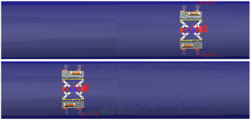
Velocity of the driving wheels and robot with a steering angle of $0^{\circ}$ : (a) angular velocity of the driving wheel, (b) translational velocity of the robot, and (c) angular velocity of the robot.

The access capabilities of the robot in the elbow are also investigated. The diameter of the straight pipe is 213 mm, the inner and outer radius of the curve 95 and 305 mm, respectively, and the length and width of the robot are 102 and 62 mm, respectively. Figure 24 shows the robot passing the elbow by using posture A, and we set the fore wheels active and leave the rear wheels passive. The angular velocities of the fore wheels are set to $720 \circ / s$ in the straight section of the pipe. When the robot enters the curved section, the speed changes from $720 \circ / s$ to $240 \circ / s$ .

Figure 24.

Robot moves in the elbow using posture A.

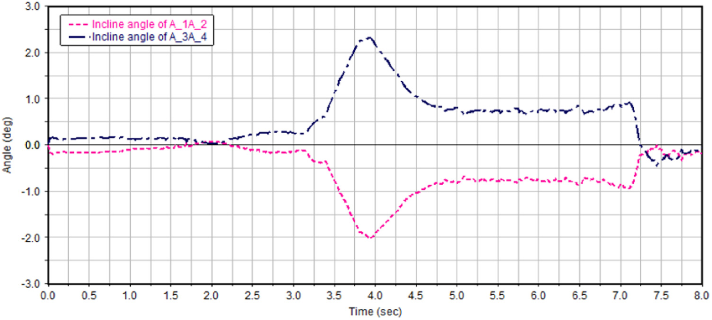
Figure 25 shows the incline angle change of $A_{1} A_{2}$ and $A_{3} A_{4}$ , and we can observe the behavior of the wall-pressing mechanism in the elbow. The robot moves in the straight pipe from 0 to 3.2 s. From 3.2 to 3.9 s, sliding joints $S_{1}$ and $S_{2}$ act to compensate for the change in the radius of the pipe. Then, the angle of $A_{1} A_{2}$ recovers to $0.8 \circ$ with respect to the robot’s center axis from 3.9 to 4.9 s. The second main process is between 4.9 to 7.1 s when the robot completely enters the curve section and moves smoothly. The incline angles of $A_{1} A_{2}$ and $A_{3} A_{4}$ remain $0.8 \circ$ . From 7.1 to 8.0 s, the robot exits the curve section, and sliding joints $S_{1}$ and $S_{2}$ compensate for the shape change of the pipe. The changes in the angle correspond with the graphs in Figure 24.

Figure 25.

Incline angle of $A_{1} A_{2}$ and $A_{3} A_{4}$ .

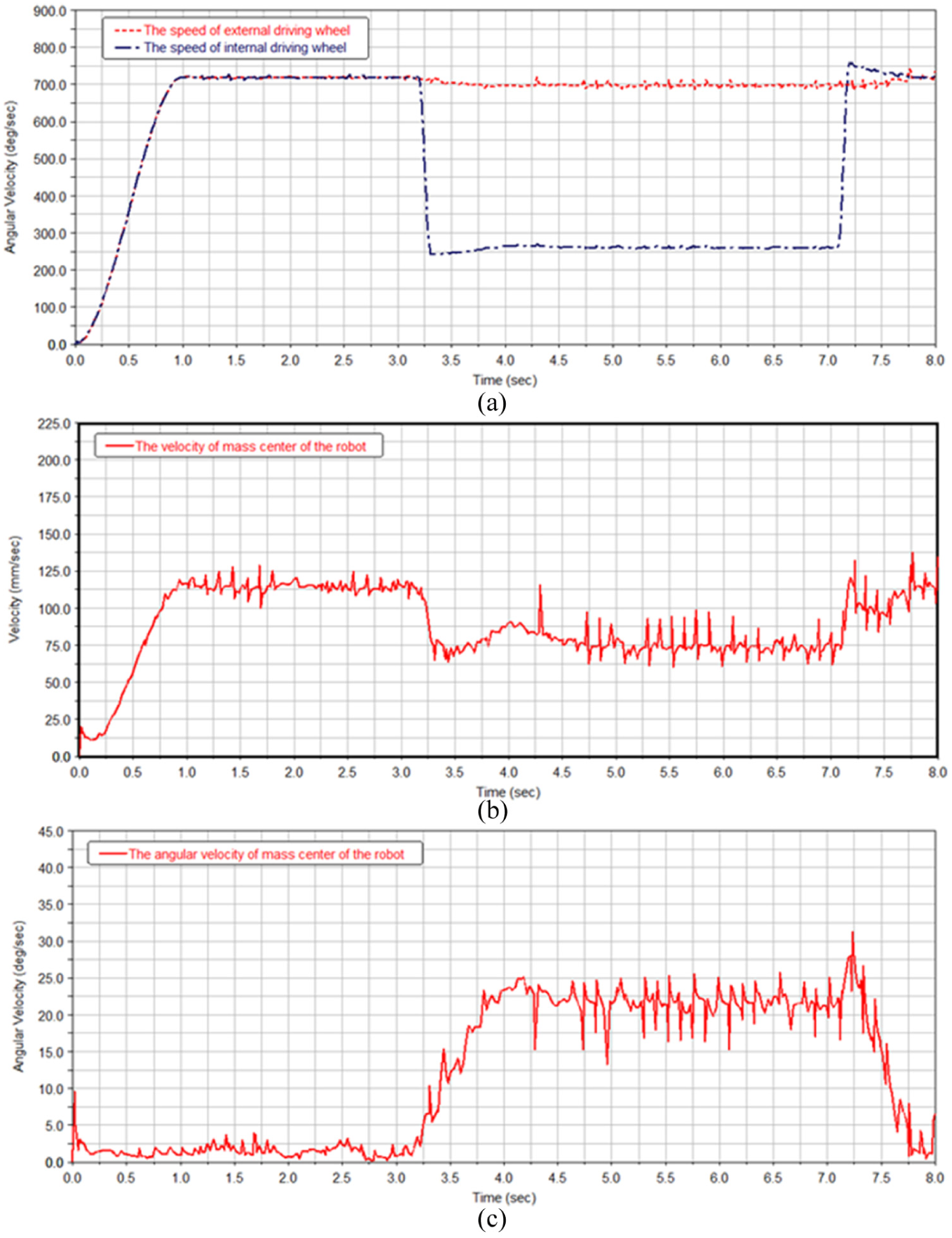
Figure 26(a) shows the velocity of the wheels in the elbow, which maintains the speed ratio in equation (14). Figure 26(b) presents the translational velocity measurement of the robot. From 0 to 3.1 s, the robot moves in the straight pipe. The velocity decreases in the curved pipe due to the speed reduction in the inner active wheels. The angular velocity in Figure 26(c) increases from $0 \circ / s$ to $22.5 \circ / s$ and becomes 0 from 7.1 to 8.0 s. These results show that when the speed ratio of the outer and inner active wheels are set appropriately, the robot can pass through the pipe smoothly.

Figure 26.

Velocity of the driving wheels and robot using posture A to pass an elbow: (a) angular velocity of the driving wheels, (b) translational velocity of the robot, and (c) angular velocity of the robot.

The robot using posture B has many benefits in square tubes and T-shape pipes. Figure 27 shows the robot passing the elbow by using posture B. In this experiment, the fore wheels are set active, and the rear ones remain passive. The steering velocities of wheels are determined according to equation (16). Figure 28(b) shows that the rear wheels follow the active wheels well, and the motion is recorded in Figure 28(a). After the robot enters the elbow, the translational velocity coordinate components vary, but the quadratic sum of these components remains stable (red line), as shown in Figure 28(c). The dark blue and blue lines in Figure 28(c) denote the velocity variations in the x and z axis directions. The x direction component decreases to zero, and the z axis value increases to 125 mm/s. The angular velocity of the robot stabilizes at $23 \circ$ when the robot is in the curve section, which is in accordance with the calculation for the above-mentioned section.

Figure 27.

Robot moves in the elbow using posture B.

Figure 28.

Velocity of the helical wheels of robot passing the elbow using posture B: (a) angular velocity of the fore wheels, (b) angular velocity of the rear wheels, (c) translational velocity of the robot, and (d) angular velocity of the robot.

When the robot passes the elbow using posture B, the curvature of the elbow is small. The driving motor only transmits power to either the driving motion or steering motion due to the one-motor design of the driving unit. Thus, the switching time of the electromagnet affects this motion conversion process. When the switching time of the electromagnet is long, the first two expressions in equation (15) can be satisfied alternately. In this case, the trajectory of the robot will not follow the centerline of the elbow strictly but will have deviations. With an increase in radius, the percentage of the deviation from radius will decrease. Thus, in the simulation of posture B in the elbow, we ignore the switching time influence of the electromagnet to investigate the common movement of this robot in the elbow. For the miniature robot passing through a small curvature, it is better to drive and steer the wheel simultaneously to achieve an ideal trajectory along the centerline of the pipe. The one-motor design can reduce the system cost effectively, and the deviation of posture B in the elbow becomes acceptable for large and curved pipes.

Conclusion

On the basis of the screw-drive principle, a robot with active-drive helical wheels was designed. Four driving units were fixed on a linkage of the wall-pressing mechanism to form the basic structure of the robot. We designed the driving units with driving and steering capability by using DC motor, gears, and a permanent magnet–type brake. The brake ring can lock either the brake main body or the wheel carrier to switch the entire driving transmission’s motion. Thus, the helical wheels acquire driving and steering capabilities. The robot operates in three motion modes according to the steering angle of the wheel and can pass complicated structures by combining these motion modes. The double slider-crank mechanism was modified to compensate for the kinematic conflict, and limit access capability of 45° was derived. For the robot moving in the elbow, we derived the motion relationship according to postures A and B. The size criterion of the robot passing in the elbow was also determined in consideration of R and D. The simulation experiments revealed that the effectiveness of the motion strategy in circular and square tube pipes. Aside from tuning the posture of the robot, the steering angle of the wheels can function as a regulator that adjusts the moving speed of the robot.

Footnotes

Handling Editor: Zhixiong Li

Declaration of conflicting interests

The author(s) declared no potential conflicts of interest with respect to the research, authorship, and/or publication of this article.

Funding

The author(s) disclosed receipt of the following financial support for the research, authorship, and/or publication of this article: This work was supported by the National Natural Science Foundation of China–Shenzhen Robot Research Program (grant no.: U1613221), the Shenzhen Fundamental Research Grant (grant no.: JCYJ20170307150346964), the Advanced Innovation Center for Intelligent Robots and Systems (grant no.: 2016IRS06), and the Shenzhen Peacock Team Program (grant no.: KQTD20140630150243062).

ORCID iD

Peng Li

Supplemental material

Supplemental material for this article is available online.

References

Appleton

Dynamic characteristics of a novel self-drive pipeline pig. IEEE T Robot 2005; 21: 781–789.

Nguyen

Kim

Rho

et al . Dynamic modeling and its analysis for pig flow through curved section in natural gas pipeline. In: Proceedings IEEE international symposium on computational intelligence in robotics and automation, Banff, AB, Canada, 29 July–1 August 2001, pp.492–497. New York: IEEE.

Choi

Youcef-Toumi

. Robot design for high flow liquid pipe networks. In: Proceedings of the IEEE/RSJ international conference on intelligent robots and systems, Tokyo, Japan, 3–7 November 2013, pp.246–251. New York: IEEE.

Roh

Choi

HR.

Differential-drive in-pipe robot for moving inside urban gas pipelines. IEEE T Robot 2005; 21: 1–17.

Oya

Okada

Development of a steerable, wheel-type, in-pipe robot and its path planning. Adv Robot 2005; 19: 635–650.

et al . Design of a mobile mechanism possessing driving ability and detecting function for in-pipe inspection. In: Proceedings of the IEEE international conference on robotics and automation, Pasadena, CA, 19–23 May 2008, pp.3992–3997. New York: IEEE.

Kwon

Lee

Whang

et al . A flat pipeline inspection robot with two wheel chains. In: Proceedings of the2011 IEEE international conference on robotics and automation, Shanghai, China, 9–13 May 2011, pp.5141–5146. New York: IEEE.

Chang

Hwang

Liu

et al . Design of a pipeline inspection robot with belt driven ridged cone shaped skate model. In: Proceedings of the IEEE international conference on robotics and biomimetics (ROBIO), Zhuhai, China, 6–9 December 2015, pp.787–792. New York: IEEE.

Kwon

BJ.

Design and motion planning of a two-module collaborative indoor pipeline inspection robot. IEEE T Robot 2012; 28: 681–696.

10.

Miyagawa

Iwatsuki

. Characteristics of in-pipe mobile robot with wheel drive mechanism using planetary gears. In: Proceedings of the international conference on mechatronics and automation, Harbin, China, 5–8 August 2007, pp.3646–3651. New York: IEEE.

11.

Enner

Rollinson

Choset

. Motion estimation of snake robots in straight pipes. In: Proceedings of the 2013 IEEE international conference on robotics and automation, Karlsruhe, 6–10 May 2013, pp.5168–5173. New York: IEEE.

12.

Melo

Paez

. Modular snake robot gaits on horizontal pipes. In: Proceedings of the IEEE/RSJ international conference on intelligent robots and systems, Vilamoura, 7–12 October 2012, pp.3099–3104. New York: IEEE.

13.

Savin

Vorochaeva

Footstep planning for a six-legged in-pipe robot moving in spatially curved pipes. In: Proceedings of the 2017 international Siberian conference on control and communications (SIBCON), Astana, Kazakhstan, 29–30 June 2017, pp.1–6. New York: IEEE.

14.

Galvez

de Santos

Pfeiffer

Intrinsic tactile sensing for the optimization of force distribution in a pipe crawling robot. IEEE/ASME T Mech 2001; 6: 26–35.

15.

Fang

Shang

Luo

et al . Development of a novel self-locking mechanism for continuous propulsion inchworm in-pipe robot. Adv Mech Eng 2018; 10: 749402.

16.

Ara

Cheng

et al . Human abdomen path-loss modeling and location estimation of wireless capsule endoscope using round-trip propagation loss. IEEE Sens J 2018; 18: 3266–3277.

17.

Song

et al . Design of in-pipe robot based on inertial positioning and visual detection. Adv Mech Eng 2016; 8: 667–679.

Supplementary Material

Please find the following supplemental material available below.

For Open Access articles published under a Creative Commons License, all supplemental material carries the same license as the article it is associated with.

For non-Open Access articles published, all supplemental material carries a non-exclusive license, and permission requests for re-use of supplemental material or any part of supplemental material shall be sent directly to the copyright owner as specified in the copyright notice associated with the article.

0.00 MB

Design and analysis of a novel active screw-drive pipe robot