Sage Journals: Discover world-class research

Abstract

The number of thermal power plants is growing due to the industry development and the growth of energy consumption. This leads to an increase in harmful emissions in the atmosphere. There is a necessity to control the emission concentration level in the areas of power plants location. The aim of this work was to study the level of pollution concentration at different distances from the source. The mathematical model and the numerical algorithm were verified by solving test problems and comparing them with the experimental data and numerical results of other authors. Furthermore, the pollution distribution in three-dimensional case was investigated in a real physical scale. CO₂ was considered as polluting gas. As a real example, the Ekibastuz SDPP-1 coal-fired thermal power plant was simulated. The remarkable feature of this thermal power plant is that the pollution emits from two chimneys of different heights (330 and 300 m). The results showed that due to the difference between chimney heights (30 m), the pollution concentration from the higher chimney dropped far away from source, than from the lower one (2160 and 1970 m, respectively). Obviously, building higher chimneys helps to reduce the harmful impact of emissions on the environment. Also, it can be used to control the emissions level at already existing power plants.

Keywords

Navier–Stokes equations mass transfer numerical simulation air pollution concentration

Introduction

Industry is developing all over the world: the number of chemical plants, thermal power plants (TPP) and nuclear power plants (NPP) is growing. They produce a large amount of pollutants. Emissions lead to various ecological problems that are harmful to human health and the environment.

TPPs generate 63% of all electricity.¹ Fuel is burned during the TPP operation and various polluting substances are dispersed in the atmosphere. About 50% of the pollution is sulphur dioxide, 30% – nitrogen oxide and 25% – fly ash.^2,3 Gaseous emissions spread through the air, chemically react and fall in the form of dry or liquid sediments on the surrounding surfaces. Depending on various factors like physical, chemical and meteorological, pollutants from power plant can settle at 500–1000 km from the source. This distance increases in proportion to the source capacity.^4–12

The study of this process in Kazakhstan is especially important. About 87% of Kazakhstan energy uses coal as fuel. According to statistics, the share of coal in the emissions production will be 66% of the total pollution by 2020. Thus, in the Republic of Kazakhstan, the energy sector is the main polluter of air.

The Gaussian model and Briggs plume rise equations are often used for pollution spread modelling.^13–22 However, they do not allow making sufficiently accurate determination of the pollution movement nature. Two-dimensional model of pollution dispersion at the earth’s boundary layer was considered by Škraba et al.¹⁴ In the previous works, Mrša and Čavrak,²³ Oliver et al.,¹⁰ and Sanín and Montero²⁴ constructed the ‘box model’ taking into account the terrain relief and wind direction. They considered SO₂ as a pollutant and used the k–ε turbulence model. Fatehifar et al.²⁵ applied the multiple cell models. Yang et al.¹² examined the capabilities of numerical simulation to describe the transport and chemical transformation of pollutants from the power plant. The simulation area is divided into two parts, based on the turbulence characteristics: JDR (jets-dominated region), which is characterized by high-pulsed jet flue gas flow, and ADR (an area with a predominance of the environment) due to the atmospheric boundary layer turbulence. Then, they tested the Reynolds-averaged Navier–Stokes equations (RANS) and large eddy simulation (LES) approaches. The results showed that LES gives more accurate results, but in comparison with RANS, it does not justify high computational costs. Toja-Silva et al.¹¹ simulated the CO₂ dispersion and compared results with the experimental measurements. They considered the TPP in the centre of the city. The TPP pollution dispersion was modelled taking into account the nearby architectural buildings and the wind direction. In this work, different values of the Schmidt number were investigated. The emission and particles distributions were investigated by Meroney.²⁶ A comparative analysis of the distribution was carried out for two cases: when buildings were located around source and when they were absent. Ghermandi et al.⁸ assessed the impact of NOx emissions on the environment from the TPP. In this paper, variable wind directions and topography relief were taken into account. Ebrahimi and Jahangirian²⁷ obtained new formulas for the Gaussian model of pollution distribution. Their results proved were closer to experimental data than the numerical results of previously known models. Barbero et al.²⁸ modelled dispersion of particles near a NPP in emergency case. Particle dispersion and deposition on buildings in urban environments were investigated by Gousseau et al.²⁹ and Kumar et al.³⁰ Olaguer et al.³¹ simulated various scenarios for the energy facilities’ operation (different capacities and regimes). They also investigated the distribution of particles and various gases.

Before simulating of such large-scale processes, it is necessary to verify the correctness of the chosen mathematical model and numerical solution method using test configurations. Later, it can be used for simulation of more complicated turbulent models. For this purpose, in this article, two-dimensional (2D) and three-dimensional (3D) test problems of the substance motion coming out of the pipe were investigated. Moreover, there are perpendicular to the main flow in the channel. Obtained results were verified and compared with the experimental data. The obtained numerical results showed closest agreement with the experimental data than the computational results of other authors.^32;–34

Then, the 3D model of the pollution distribution in real scales was considered. The obtained results were also compared with the data of other authors.⁵ CO₂ was considered as a pollution substance. Then, simulation of atmospheric pollution by the Ekibastuz SDPP-1 (Ekibastuz State District Power Plant-1) was carried out. Ekibastuz SDPP-1 is the largest TPP in the Republic of Kazakhstan, which is located on the northern side of Zhyngyldy lake shore, at 16 km north from the Ekibastuz city, Pavlodar region (see Figure 1). Operation capacity of Ekibastuz SDPP-1 is about 3500 MW. Dimensions of the main building: length – 500 m, width – 132 m and height – 64 m. Height of chimneys: 300 m (built in 1980) and 330 m (built in 1982). The difference between chimneys made it possible to study the source height influence on the pollution dispersion. According to the obtained numerical results, increase in chimney height reduces the emission concentration.

Figure 1.

Ekibastuz SDPP-1, Pavlodar region, Kazakhstan.

Mathematical model

Margason³⁵ gave a detailed description of the latest works devoted to the study of the jet distribution in the crossflow. Authors numerically simulated the velocity field in previous papers.^36–42 The passive scalar mass fraction was considered in previous works.^43–45 Numerical algorithms are often used to solve these problems. In many previous works,^46–50 RANS were used and the numerical results were compared with the experimental data. The good correspondence between numerical solutions (direct numerical simulation [DNS] method) and experiments was obtained by Chochua et al.⁵¹, Acharya et al.⁵² and Camussi et al.⁵³ These problems were also investigated in previous works.^54–57 However, the DNS method requires large computational costs, which is unacceptable for solving large-scale problems in real scales.^58–60 As a result, in this article, the k–ε turbulence model was used.

The CFD simulations of such processes are based on the Navier–Stokes equations (momentum and continuity equations)^61–64

\frac{\partial u_{j}}{\partial x_{j}} = 0

(1)

\frac{\partial ρ u_{i}}{\partial t} + \frac{\partial}{\partial x_{j}} (ρ u_{i} u_{j}) = - \frac{\partial p^{'}}{\partial x_{i}} + \frac{\partial}{\partial x_{j}} [μ_{e f f} (\frac{\partial u_{i}}{\partial x_{j}} + \frac{\partial u_{j}}{\partial x_{i}})] - ρ \vec{g} \overset{⌢}{n}

(2)

where $μ_{eff}$ is the effective viscosity and $p'$ is the modified pressure. Here $p' = p + (2 / 3) ρ k + (2 / 3) μ_{eff} (\partial u_{k} / \partial x_{k})$ and $μ_{eff} = μ + μ_{t}$ , where $μ_{t} = C_{μ} ρ (k^{2} / ε)$ is the turbulence viscosity

\frac{\partial k}{\partial t} + \frac{\partial}{\partial x_{j}} (u_{j} k) = \frac{\partial}{\partial x_{j}} [(μ + \frac{μ_{t}}{σ_{k}}) \frac{\partial k}{\partial x_{j}}] + P_{k} - ρ ε + P_{kb}

(3)

\frac{\partial ε}{\partial t} + \frac{\partial}{\partial x_{j}} (u_{j} ε) = \frac{\partial}{\partial x_{j}} [(μ + \frac{μ_{t}}{σ_{ε}}) \frac{\partial ε}{\partial x_{j}}] + \frac{ε}{k} (C_{ε 1} P_{k} - C_{ε 2} ρ ε + C_{ε 1} P_{ε b})

(4)

The term $P_{k}$ represents the turbulence kinetic energy generation due to the mean velocity gradients

P_{k} = μ_{t} (\frac{\partial u_{i}}{\partial x_{j}} + \frac{\partial u_{j}}{\partial x_{i}}) \frac{\partial u_{i}}{\partial x_{j}} - \frac{2}{3} \frac{\partial u_{k}}{\partial x_{k}} (3 μ_{t} \frac{\partial u_{k}}{\partial x_{k}} + ρ k)

(5)

$P_{kb}, P_{ε b}$ represent the buoyancy forces, where $P_{k b} = - (μ_{t} / ρ σ_{ρ}) ρ β g_{i} (\partial T / \partial x_{i})$ and $P_{ε b} = C_{3} max (0, P_{kb})$ . Here, $β$ is the thermal expansion coefficient, $σ_{ρ} = 0.9$ , $C_{ε 1}, C_{ε 2}, σ_{k}, σ_{ε}$ are constants.

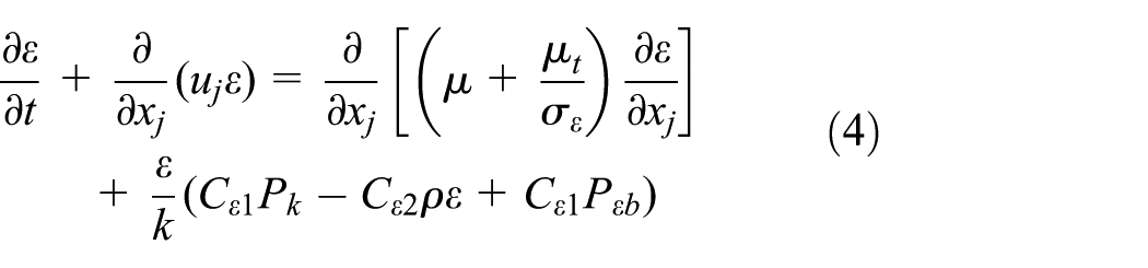
Species transport equations

Transport equations were used to solve chemical species transport conservation. ANSYS Fluent simulates the local mass fraction of each species $Y_{i}$ , by solving the convection–diffusion equation for the ith species

\frac{\partial}{\partial t} (ρ Y_{i}) + \nabla \cdot (ρ \vec{u} Y_{i}) = - \nabla \cdot ((ρ D_{i, m} + \frac{μ_{t}}{S c_{t}}) \nabla Y_{i}) + R_{i} + S_{i}

(6)

where $R_{i}$ is the net production rate of species i by chemical reaction and $S_{i}$ is the creation rate by addition from the dispersed phase, $S c_{t} = μ_{t} / ρ D_{t}$ is the turbulent Schmidt number ( $μ_{t}$ is the turbulent viscosity and $D_{t}$ is the turbulent diffusivity). By default, $S c_{t}$ is 0.7, but in this article, it was set as 1, as in the papers by Falconi et al.³² and Schonauer and Adolph.³³

Energy equation looks like

\frac{\partial}{\partial T} (ρ E) + \nabla \cdot (\vec{v} (ρ E + p)) = \nabla \cdot (k_{e f f} \nabla T - \sum_{j} h_{j} {\vec{J}}_{j} + ({\bar{\bar{τ}}}_{e f f} \cdot \vec{v})) + S_{h}

(7)

where $k_{eff} = k + k_{t}$ is the effective conductivity, where $k_{t}$ is the turbulent thermal conductivity, which was defined according to the turbulence model, ${\vec{J}}_{j}$ is the diffusion flux of species j. The first three components in the parentheses on the right-hand side (RHS) of equation (7) express the energy transfer due to conduction, the species diffusion and the viscous dissipation, respectively. $S_{h}$ takes into account the energy of chemical reaction

E = h - \frac{p}{ρ} + \frac{v^{2}}{2}

(8)

where $h = \sum_{j} Y_{j} h_{j} + (p / ρ)$ , $Y_{j}$ is the mass fraction of species j, $h_{j} = \int_{T_{ref}}^{T} c_{p, j} dT$ , where $T_{ref} = 298.15 K$ .

For the arbitrary scalars $ϕ_{k}$ , ANSYS Fluent solves the following equations

\frac{\partial ρ ϕ_{k}}{\partial t} + \frac{\partial}{\partial x_{i}} (ρ u_{i} ϕ_{k} - Γ_{k} \frac{\partial ϕ_{k}}{\partial x_{i}}) = S_{ϕ_{k}}, k = 1, \dots, N

(9)

where $Γ_{k}$ and $S_{ϕ_{k}}$ are the diffusion coefficient and the source term, respectively, which supplied for each of the N scalar equations. Note that $Γ_{k}$ is determined as a tensor if it can be determined as anisotropic diffusivity.

For the steady case (stationary), ANSYS can solve one of the three equations, depending on the numerical method which is used to compute the convective flux term:

If it is possible to neglect convective flux term, ANSYS Fluent will solve the following equation

- \frac{\partial}{\partial x_{i}} (Γ_{k} \frac{\partial ϕ_{k}}{\partial x_{i}}) = S_{ϕ_{k}}, k = 1, \dots, N

(10)

If convective flux term will be taken into account, the following equation will be like that

\frac{\partial}{\partial x_{i}} (ρ u_{i} ϕ_{k} - Γ_{k} \frac{\partial ϕ_{k}}{\partial x_{i}}) = S_{ϕ_{k}}, k = 1, \dots, N

(11)

It is also possible to specify a user-defined function (UDF), which will use convective flux term in the simulation. In this case, it will looks like in this form

F = \int_{S} ρ \bar{u} \cdot d \bar{S}

(12)

where $d \bar{S}$ is the face vector area.

2D test problem

The present test problem was computed before by Falconi et al.³² and Schonauer et al.³³ Here, a laminar jet inlet from a pipe, to the main crossflow, is located perpendicular to the jet (see Figure 2). The chemical component B enters perpendicular to the flow (input 2), component A – by the side of main channel (input 1). The components of species A and B are reacting and produce species C.

Figure 2.

The dimensions of the computational domain (m).

Computational domain and grid

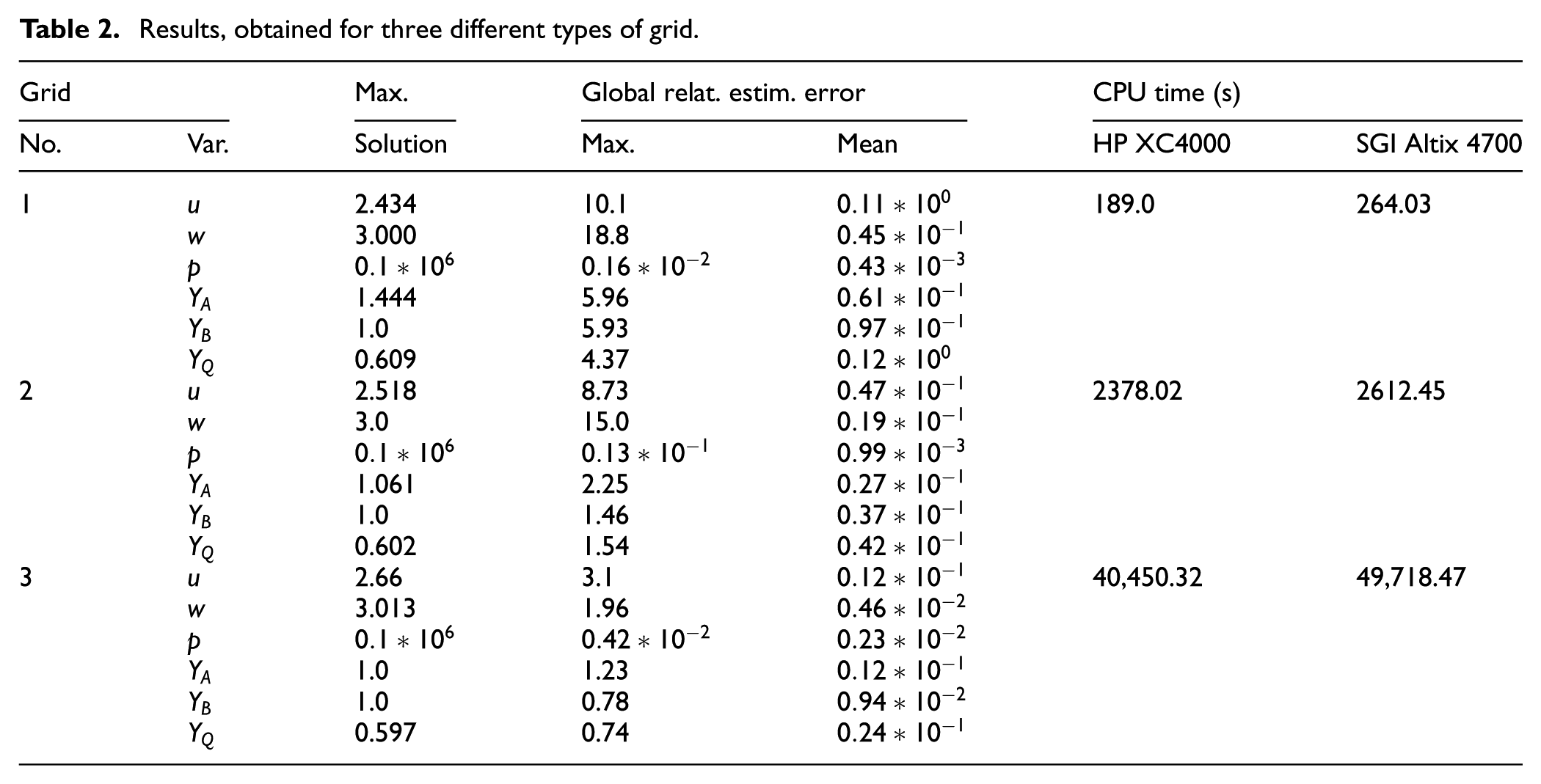
Figure 2 shows the dimensions of computational domain. It is assumed an incompressible fluid with Reynolds number 25.^32,33 The computational grid in the main part of channel consists of 2561 × 641 dimensions, the dimensions of the pipe: 161 × 321. As a result, the number of nodes are 1,693,121 (see Table 1, line 3). The choice of these parameters for the grid construction is based on the simulation results.³³ In this article, the sensitivity of the numerical results to the computational grid with various nodes amount is investigated to obtain an optimal grid arrangement. It is obviously that the computational grid described in Table 1, line 3, has a good arrangement between the CPU time and the accuracy prescribed in the test problem (see Table 2). Increasing the number of grid elements allow to reduce the global maximum relative error.

Table 1.

Three various variants of simulation grids.

Grid	Dimensions		Number of
No.	Main channel	Pipe	Nodes	Elements	Unknowns
1	641 × 161	41 × 81	106,481	211,200	638,886
2	1281 × 321	81 × 161	424,161	844,800	2,544,966
3	2561 × 641	161 × 321	1,693,121	3,379,200	10,158,726

Table 2.

Results, obtained for three different types of grid.

Grid		Max.	Global relat. estim. error		CPU time (s)
No.	Var.	Solution	Max.	Mean	HP XC4000	SGI Altix 4700
1	u w p $Y_{A}$ $Y_{B}$ $Y_{Q}$	2.434 3.000 $0.1 * 10^{6}$ 1.444 1.0 0.609	10.1 18.8 $0.16 * 10^{- 2}$ 5.96 5.93 4.37	$0.11 * 10^{0}$ $0.45 * 10^{- 1}$ $0.43 * 10^{- 3}$ $0.61 * 10^{- 1}$ $0.97 * 10^{- 1}$ $0.12 * 10^{0}$	189.0	264.03
2	u w p $Y_{A}$ $Y_{B}$ $Y_{Q}$	2.518 3.0 $0.1 * 10^{6}$ 1.061 1.0 0.602	8.73 15.0 $0.13 * 10^{- 1}$ 2.25 1.46 1.54	$0.47 * 10^{- 1}$ $0.19 * 10^{- 1}$ $0.99 * 10^{- 3}$ $0.27 * 10^{- 1}$ $0.37 * 10^{- 1}$ $0.42 * 10^{- 1}$	2378.02	2612.45
3	u w p $Y_{A}$ $Y_{B}$ $Y_{Q}$	2.66 3.013 $0.1 * 10^{6}$ 1.0 1.0 0.597	3.1 1.96 $0.42 * 10^{- 2}$ 1.23 0.78 0.74	$0.12 * 10^{- 1}$ $0.46 * 10^{- 2}$ $0.23 * 10^{- 2}$ $0.12 * 10^{- 1}$ $0.94 * 10^{- 2}$ $0.24 * 10^{- 1}$	40,450.32	49,718.47

Boundary conditions and flow characteristics

The simulations were carried out using ANSYS Fluent, where all simulations are made in physical sizes. That is why in this article, the physical parameters have been specified, not dimensionless parameters.

The species transport equations have been applied for calculating the mass fraction distribution. The SIMPLE algorithm with finite volume method was chosen for the numerical solution. Convergence condition was set as $ε = 0.00001$ . The jet to crossflow velocity ratio is expressed as $R = U_{jet} / U_{crossflow} = 1.5$ . Damköhler number is set as 1. The flow is considered as incompressible due to the low velocity and small Mach number.

Boundary conditions in ANSYS were set as follows: for the inlet 1 and inlet 2 –‘Velocity inlet’, for the outlet –‘Pressure-outlet’, for the walls –‘Wall’. It means that for the main channel outlet boundary is applied gradient for all quantities equal to zero. For top and bottom walls, there is no slip for the velocities and wall-normal gradient for the scalar components.

Different types of the u velocity profile (where u– horizontal velocity component, $r = y$ ) were considered for main channel inlet (inlet 1; see Table 3).

Table 3.

Various velocity profiles.

$u 1$	$u 2$	$u 3$	$u 4$
$u^{*}$	$u^{*} (1 - e^{- 4.5 (1 - \frac{r^{2}}{4})})$	$u^{*} (1 - e^{- 5 (1 - \frac{r^{2}}{4})})$	$u^{*} (1 - e^{- 5.5 (1 - \frac{r^{2}}{4})})$

Thus, the influence of various pre-exponential coefficients on the flow nature was investigated. $u^{*}$ varies depending on the selected material. The oxygen was set as A and B substances. Required Reynolds number is $Re = ρ u_{crossflow} D / μ = 25$ , taking into account that dynamic viscosity of the oxygen, which is $μ = 1.919 e - 05 kg m^{2} / s$ and density is $ρ = 1.299874 kg / m^{3}$ , the velocity was set as $u^{*} = 0.000369074233 m / s$ .

Other parameters for crossflow inlet were set as constants: $w = 0$ (vertical velocity component), $Y_{A} = 1$ , $Y_{B} = 0$ .

For the entry of pipe (inlet 2), $Y_{A} = 0$ , $Y_{B} = 1$

u = 0, w = 2 R u^{*} (1 - 4 l^{2}), l = x

(13)

The hydraulic diameter was $D = 1 m$ . The diffusion coefficient was defined as $0.67737051 m^{2} / s$ to obtain required Schmidt number $(S c_{t} = 1)$ .

Comparison of numerical results

The numerical results and the comparative analysis for the velocity field and mass fraction are presented below. The results were compared with the computational solutions of Schonauer et al.³³ and showed good coincidence. Figure 3 illustrates the comparison of velocity streamlines for the flow through the computational domain (initial velocity profile u3, see Table 3). The length of the vortex after the pipe in both cases is approximately l = 5.9D.

Figure 3.

Comparison of streamlines, from top to bottom: the results of Schonauer et al.³³ and the results of this article.

Figure 4 presents a comparative analysis of the species transport, where C1, C2 and C3 – the mass fraction of A, B and C substances, respectively. Species mass fraction can be defined as the species mass per unit the mixture mass (kg of species in 1 kg of the mixture), that is, dimensionless quantity. The results also showed a good coincidence.

Figure 4.

Comparison of contour plots for mass fractions, from top to bottom: the results of Schonauer et al.³³ and the results of this article: (a) product A, (b) product B and (c) reaction product C.

Figure 5 shows product concentration profiles. Data were taken at various sections (x/D = 0.0 and x/D = 3.0). Difference between the $u 2, u 3, and u 4$ profiles is almost negligible and the influence of the pre-exponential coefficient is small. However, the $u 1$ profile is different from them. It follows that it is important to set the velocity profile as a parabolic function, rather than constant, since it significantly affects the result.

Figure 5.

Various mass fraction profiles for the reaction product C at different distances: (a) x/D = 0.0 and (b) x/D = 3.0 (m).

3D test problem

An experimental study for 3D test problem was conducted in a low-speed wind tunnel on a row of six rectangular jets injected at the perpendicular to the crossflow.^34,65 Using a three-component Doppler velocimeter laser, which is operating in coincidence mode were measured mean velocity component and six flow stresses. Seeding of jet and crossflow air was achieved with the smoke generator. For the detailed measurements of the flow, accomplished visualization was used by transmitting the laser beam through a cylindrical lens, which is generates an intense sheet of light.

Computational domain and grid

The computational domain included the jet and the flat plate which is located above the jet. For simulation, the square jet was used and jet diameter was D, which was used as the length unit (Figure 6). The origin of the coordinate system was located at the jet exit centre. The calculation area of the test problem is a 3D channel with the pipe entering into it. The height of the crossflow channel is 20D, jet channel length is 5D, the length of the crossflow channel is 45D, the width is 3D and the centre of the pipe located at 5D from the inlet (see Figure 6). Number of grid points was as follows: main channel 230 × 100 × 21 and jet channel 7 × 30 × 7 nodes. Grid was unstructured, and the total number of nodes was 533,697.

Figure 6.

Configuration of computational domain.

Boundary conditions and flow characteristics

The ratio of the jet velocity to the crossflow velocity is denoted by R and is expressed as follows

R = \frac{V_{jet}}{V_{crossflow}}

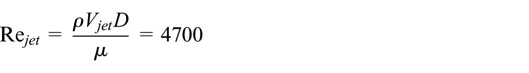
In the paper by Keimasi and Taeibi-Rahni,⁶⁵ various ration of the jet R (0.5, 1.0 and 1.5) was considered. In this article, R = 0.5 was considered, that is why the jet velocity was 5.5 m/s, crossflow velocity was 11 m/s. Water was chosen as the material of the crossflow and jet fluid. The jet diameter was D = 12.7 mm. Based on the above data, the Reynolds number is defined as follows

{Re}_{jet} = \frac{ρ V_{jet} D}{μ} = 4700

Five types of boundary conditions were used: inlet, outlet, no flux, wall and periodic. According to the experimental data, the boundary layer thickness is 2D. To describe the initial crossflow velocity profile in the boundary layer, 1/7 power law wind profile was used

\frac{u}{u_{r}} = {(\frac{z}{z_{r}})}^{α}

Here, u is the wind velocity at height z and $u_{r}$ is the known wind velocity at a reference height $z_{r}$ . $α$ is the obtained empirically coefficient, which varies depending on the atmosphere stability. Here, $α = 1 / 7$ for neutral stability conditions. Uniform velocity (11 m/s) was defined above the boundary layer 2D.

Comparison of numerical results

Figure 7 shows a comparison of the numerical results for the horizontal velocity component at jet centre plane (z/D = 0) with experimental data and computational solutions of other authors (R = 0.5). The red solid line marks the results of this article, round-shaped marks represent the results of experimental data,³⁴ and the rest of the lines illustrate computational solutions of other authors.⁶⁵ The results for the shear stress transport (SST) model are shown by blue squares.

Figure 7.

Comparison of results for the horizontal velocity component at jet centre plane (z/D = 0) for R = 0.5 with the computational data⁶⁵and the experimental data:³⁴ (a) x/D = 0 and (b) x/D = 3.

Comparative analysis showed that the k–ε model and the SIMPLE algorithm with finite volume method yield closest results to the experimental data (see Figure 7(b)). The solutions obtained in this article turned out to be more accurate than those computational solutions obtained by other authors.⁶⁵ Values of the red line (u/V_jet) at y/D = 0 close to zero, when other results close to ∼0.5–0.7. This is more accurate from a physical point of view, since it is a near-wall field. Moreover, in the interval y/D∼0.5–1.5, it is noticeable that the current simulation results are much closer to the experimental data than the others authors. One of the reasons is the quality of the grid: in this article, unstructured grid was used, the number of nodes was 533,697, while in the paper by Keimasi and Taeibi-Rahni,⁶⁵ structured grid was used and the number of nodes was 265,000.

3D problem in real physical scale

In this section, a 3D problem in real physical scale is presented. The comparative analysis with paper by Zavila⁵ was carried out. The results of the work by Zavila⁵ had been verified by an experiment performed in a low-speed wind tunnel.

Computational domain and grid

The 3D box with a chimney was chosen as the computational domain. Emissions are released from the chimney hole. Figure 8 shows the geometry and grid of computational domain. The dimensions are described in Table 4. For accurate simulation, the grid was nonuniform and was clustered near the wall, around the chimney exit and along the trajectory of pollution motion. The total number of 3D cells is 568,486. The test problems were solved using the standard k–ε model, but in present investigation, it was used RNG k–ε to compare the results with paper by Zavila.⁵ According to Chang et al.⁶⁶ and Saeed et al.,⁶⁷ standard k–ε and Re-Normalisation Group (RNG) k–ε turbulent models give almost the same results.

Figure 8.

3D problem in real physical scale: (a) the geometry of simulating field and (b) the computational unstructured mesh.

Table 4.

Geometry parameters.

	Geometry dimensions (m)	Stack dimensions (m)	Inlet dimensions (m)	Coordinates of stack (m)
1:1	X = 2000 Y = 1500 Z = 1500	X = 3.5 Y = 200 Z = 3.5	X = 3.5 Y = 3.5	X = 500 Y = 0.0 Z = 50

Boundary conditions and flow characteristics, comparison of numerical results

Boundary conditions for wind inlet were set as the ‘Velocity inlet’ and ‘Wall’ for chimney walls, the chimney hole and the ground; ‘Pressure Outlet’ for the outlet of channel; and ‘Symmetry’ boundary conditions were used for the front, back and top walls.

Zavila⁵ considered the helium dispersion for different wind velocities: 1, 3 and 5 m/s. For comparison, the third case was chosen (v_air = 5 m/s; see Figure 9). As in the test problem, species transport model was applied for pollution movement simulation. It was assumed that discharge substances do not react with air. The influence of gravity was taken into account. The temperature and convergence criterion were set as 300 K $(27^{\circ} C)$ and $ε = 0.0001$ , respectively. All parameters were defined similar to the paper by Zavila.⁵ Figure 9 shows good correspondence with the previous results.⁵ Results were visualized as pollutant concentrations isosurfaces; the maximum mass fraction value was set as 0.00003.

Figure 9.

The helium distribution numerical results. From left to right: results of Zavila⁵ and present results (wind velocity is 5 m/s).

Ekibastuz State District Power Plant-1 (Ekibastuz SDPP-1)

Next, the real physical model of the pollution distribution from Ekibastuz SDPP-1 (Ekibastuz city) was considered. At this TPP, pollution emits from two chimneys (300 and 330 m). The distance between the chimneys is about 250 m (see Figure 10). Diameters of chimney holes are 10 m. Two cases with different wind velocities were tested: 1.0 and 1.5 m/s (Figure 11). Velocity of pollutants from chimneys: 5 m/s. To describe the boundary layer, the following initial wind velocity profile was applied $v_{x} = v_{wind} \cdot (0.2371 \cdot \ln (Y + 0.00327) + 1.3571) (m s^{- 1})$ .

Figure 10.

Satellite image of Ekibastuz SDPP-1 thermal power plant. Distance between the chimneys is 250 m.

Figure 11.

CO₂ motion analysis (Ekibastuz SDPP-1) for various wind velocities: (a) 1.0 m/s and (b) 1.5 m/s.

CO₂ was considered as a pollutant in this case (see Figure 11). In the figure, it is obvious that at higher wind velocity, pollution settles on the ground much farther from the source than at low wind velocities. Also, the distances for different chimney heights from the pollution source were determined. For this purpose, mass fraction profiles from two chimneys were compared at different distances from the source (wind velocity 1.5 m/s): 1750 and 2150 m (see Figure 12).

Figure 12.

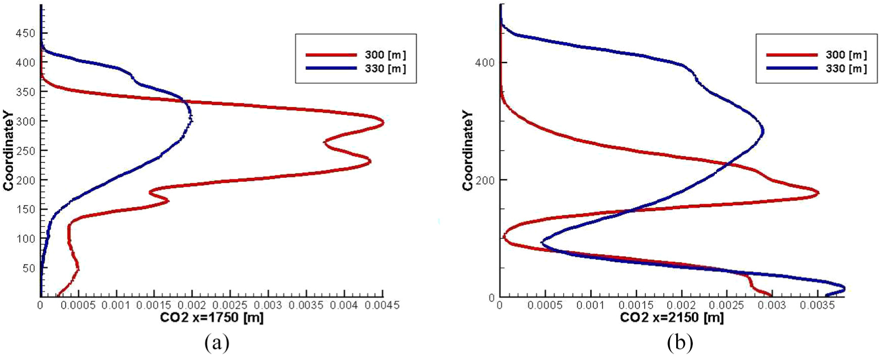
Comparison of CO₂ mass fraction profiles at various distances for two different height chimneys (300 and 330 m): (a) 1750 m, (b) 2150 m and wind velocity: 1.5 m/s.

Figure 12 clearly shows that contamination from a smaller pipe (300 m) settles closer to the source. At the distance of 1750 m from the chimney with source, a small amount of CO₂ concentration is already observed on the ground surface. On the contrary, pollution from a higher chimney at this distance still does not reach the ground in large quantities and is practically zero. At an altitude of 150–350 m, large emission concentrations are observed for a chimney with height 300 m, compared to a chimney with height 330 m. This is due to the fact that in this interval, contaminants from a smaller chimney are added with contaminants from the high chimney, since the distance between the two chimneys is only 250 m and the emissions can dissipate well. At a distance of 2150 m, the concentration of contaminants from both chimneys is already settling. Generally, pollution concentration (CO₂) tend to be higher at ground level than at chimney height (∼300 m), where the diffusion effect is smoother. This effect is associated with turbulent eddy dissipation. Toja-Silva et al.¹¹ showed that the pollution concentrations change trajectory and drop below towards the ground at a distance of about 500 m from the chimney. At a distance of about 700 m from the power plant, high concentrations are observed at ground level. However, this phenomenon is also observed in this work, but there are differences in pollution dropping distances because of the various chimney heights: in the paper by Toja-Silva et al.,¹¹ the TPP has the chimney height about 90 m, but Ekibastuz SDPP-1 TPP has the chimney height 300 m for the first one and 330 m for the second one.

Conclusion

The aim of this work was to identify the distance from the chimney with source at which the contamination settles and the factors affecting it. For this purpose, a numerical simulation of gaseous pollutant plume motion and dispersion was conducted in real atmospheric conditions. Moreover, in this work, additional dispersion model did not apply. The influence of various wind velocities and chimney dimensions was investigated.

In the beginning, numerical methods were tested using 2D and 3D test problems. The jet, entering from the channel, perpendicular to the main flow, was considered in sections ‘2D test problem’ and ‘3D test problem’. A comparative analysis of obtained numerical results with the numerical data of other authors^32,33,65 showed that the results are in good agreement with each other. It should be noted that these computational results have been found to be much closer to the experimental data than the computational results obtained by other authors⁶⁵ due to the improved grid. As a result, it was revealed that the initial velocity profile has a significant influence on the further character of impurity distribution.⁶⁵

Next, a 3D simulation of pollution distribution in real physical scale was conducted in section ‘3D problem in real physical scale’. The distribution of He was considered. The fine grid was constructed near the ground, around the chimney exit and along the pollution motion trajectory. It allowed to minimize simulations cost and focus on areas of interest.

In section ‘Ekibastuz State District Power Plant-1 (Ekibastuz SDPP-1)’, the real physical model of the pollution distribution from Ekibastuz SDPP-1 was considered. From the results it is obvious that the height of the chimneys significantly influences the pollution distribution. Building of higher chimneys is more appropriate for the ecology safety. Safe distances (1750 m for the first chimney (300 m) and 2150 m for the second chimney (330 m)) were also determined from the falling concentration of the two chimneys of the TPP.

Future research should continue to examine knowledge in describing distribution of species in the air at various distances. It will help to determine optimal location of TPPs with respect to human settlements in advance. This will help to minimize the damage to flora and fauna caused by emissions from the chimneys of TPP.

Footnotes

Handling Editor: Bo Yu

Author note

Alibek Issakhov is also affiliated with Kazakh-British Technical University, Almaty, Kazakhstan.

Declaration of conflicting interests

The author(s) declared no potential conflicts of interest with respect to the research, authorship and/or publication of this article.

Funding

The author(s) received no financial support for the research, authorship and/or publication of this article.

ORCID iD

Alibek Issakhov

References

El-Sharkawi

MA.

Electric energy – an introduction. 3rd ed.New York: CRC Press/Taylor & Francis Group, 2013, p.53

Abbaspour

Javid

Moghimi

et al . Modeling of thermal pollution in coastal area and its economical and environmental assessment. Int J Environ Sci Tech 2005; 2: 13–26.

US Environmental Protection Agency. Clean air markets division, 2016, https://ampd.epa.gov/ampd/:

US environmental health, and safety guidelines for thermal power plants. Washington, DC: International Finance Corporation, 2017.

Zavila

. Physical modeling of gas pollutant motion in the atmosphere. In: Liu

(ed.) Advances in modeling of fluid dynamics. London: InTech, 2012. pp. 51–78.

Goyal

Kumar

. Mathematical modeling of air pollutants: an application to Indian urban city. In: Popovic

(ed.) Air quality-models and applications. London: InTech, 2011. pp. 101–130.

Kozic

MS.

A numerical study for the assessment of pollutant dispersion from Kostolac B power plant to Viminacium for different atmospheric conditions. Thermal Sci 2015; 19: 425–434.

Ghermandi

Fabbi

Arvani

et al . Impact assessment of pollutant emissions in the atmosphere from a power plant over a complex terrain and under unsteady winds. Sustainability 2017; 9: 2076.

Srinivas

Rakesh

Baskaran

et al . Source term assessment using inverse modeling and environmental radiation measurements for nuclear emergency response. Air Qual Atmos Health 2017; 10: 1077–1087.

10.

Oliver

Montero

Montenegro

et al . Adaptive finite element simulation of stack pollutant emissions over complex terrains. Energy 2013; 49: 47–60.

11.

Toja-Silva

Chen

Hachinger

et al . CFD simulation of CO₂ dispersion from urban thermal power plant: analysis of turbulent Schmidt number and comparison with Gaussian plume model and measurements. J Wind Eng Ind Aerodynam 2017; 169: 177–193.

12.

Yang

Zhang

KM.

CFD-based turbulent reactive flow simulations of power plant plumes. Atmospheric Environment 2017; 150: 77–86.

13.

Mrša

Čarija

. Maximum air pollution simulation using genetic algorithm. In: 4th international congress of Croatian society of mechanics, 18–20 September 2003, Bizovac, pp.18–20.

14.

Škraba

Stojanović

Amicis

et al . Integrating air-pollution dispersion simulation models and GIS for urban air-pollution emergency management. In: 7th Vienna conference on mathematical modeling, 14–17 February 2012, Vienna.

15.

Fatehifar

Elkamel

Alizadeh Osalu

et al . Developing a new model for simulation of pollution dispersion from a network of stacks. Appl Mathemat Comput 2008; 206: 662–668.

16.

Daly

Zannetti

. Air pollution modeling – an overview. In: Zannetti

Al-Ajmi

Al-Rashied

(eds) Ambient air pollution. The Arab School for Science and Technology (ASST) and The EnviroComp Institute, 2007. pp. 15–28.

17.

Igbokwe

Azubuike

Nwufo

et al . Critical review and analysis of general pollutants associated with thermal power plants in Nigeria and control techniques. Res Rev: J Eng Tech 2016; 5. RROIJ Group.

18.

Rafee

Martins

Kawashima

et al . Contributions of mobile, stationary and biogenic sources to air pollution in the Amazon rainforest: a numerical study with the WRF-Chem model. Atmos Chem Phys 2017; 17: 7977–7995.

19.

Tomiyama

Kobayashi

Tanabe

et al . Temporal emission distribution corresponding to operating quantity in thermal power plant. J Japan Soc Atmos Environ 2016; 51: 124–131.

20.

Muhaimin

MSE

Suratman

. Air pollution simulation from Cirebon power plant activity. Jurnal Eksakta 2016; 15: 14–22.

21.

Mou

B-J

Zhao

D-X

et al . Numerical simulation of the effects of building dimensional variation on wind pressure distribution. Eng Appl Comput Fluid Mech 2017; 11: 293–309.

22.

Muhaimin

MSE

. Air pollution simulation based on different seasons. J Phys Conf Ser 2017; 795: 012072.

23.

Mrša

Čavrak

. Modeling of dispersion and diffusion of pollutants from industrial chimney stacks in Rijeka refinery. In: 4th international congress of Croatian society of mechanics, 18–22 September 2003, Bizovac, pp.18–20.

24.

Sanín

Montero

A finite difference model for air pollution simulation. Adv Eng Software 2007; 38: 358–365.

25.

Fatehifar

Elkamel

Taheri

MATLAB-based modeling and simulation program for dispersion of multipollutants from an industrial stack for educational use in a course on air pollution control. Comp Appl Eng Educ 2006; 14: 300–312.

26.

Meroney

RN.

CFD prediction of cooling tower drift. J Wind Eng Ind Aerodyn 2006; 94: 463–490.

27.

Ebrahimi

Jahangirian

New analytical formulations for calculation of dispersion parameters of Gaussian model using parallel CFD. Environ Fluid Mech 2013; 13: 125–144.

28.

Barbero

Cuadra

Domingo

et al . Investigation of the near-range dispersion of particles unexpectedly released from a nuclear power plant using CFD. Environ Fluid Mech 2015; 15: 67–83.

29.

Gousseau

Blocken

Stathopoulos

et al . CFD simulation of near-field pollutant dispersion on a high-resolution grid: a case study by LES and RANS for a building group in downtown Montreal. Atmos Environ 2011; 45: 428–438.

30.

Kumar

Feiz

Ngae

et al . CFD simulation of short range plume dispersion from a point release in an urban like environment. Atmos Environ 2015; 122: 645–656.

31.

Olaguer

Knipping

Shaw

et al . Microscale air quality impacts of distributed power generation facilities. J Air Waste Manag Assoc 2016; 66: 795–806.

32.

Falconi

Denev

Frohlich

et al . A test case for microreactor flows – a two-dimensional jet in crossflow with chemical reaction (2d test case for microreactor flows, Internal Report), July20, http://www.ict.uni-karlsruhe.de/index.pl/themen/dns/index.html

33.

Schonauer

Adolph

Results of the Snuffle Problem Denev by the FDEM program. Abschlussbericht des Verbundprojekts FDEM, UniversitË at Karlsruhe, Karlsruhe, 2005.

34.

Ajersch

Zhou

Ketler

et al . Multiple jets in a crossflow: detailed measurements and numerical simulations. In: International gas turbine and aeroengine congress and exposition (ASME Paper 95-GT-9), 5–8 June, Houston, TX, pp.1–16.

35.

Margason

. Fifty years of jet in crossflow research. In: Proceedings of the AGARD symposium on computational and experimental assessment of jets in crossflow, Winchester, April 1993, AGARD CP 534.

36.

Kamotani

Greber

Experiments on turbulent jet in a crossflow. AIAA J 1972; 10: 1425–1429.

37.

Fearn

Weston

RP.

Vorticity associated with a jet in crossflow. AIAA J 1974; 12: 1666–1671.

38.

Andreopoulos

Rodi

Experimental investigation of jets in a crossflow. J Fluid Mech 1984; 138: 93–127.

39.

Krothapalli

Lourenco

Buchlin

JM.

Separated flow upstream of a jet in a crossflow. AIAA J 1990; 28: 414–420.

40.

Fric

Roshko

Vortical structure in the wake of a transverse jet. J Fluid Mech 1994; 279: 1–47.

41.

Kelso

Lim

Perry

AE.

An experimental study of round jets in cross-flow. J Fluid Mech 1996; 306: 111–144.

42.

Muppidi

Mahesh

Direct numerical simulation of round turbulent jets in crossflow. J Fluid Mech 2007; 574: 59–84.

43.

Smith

Mungal

MG.

Mixing, structure and scaling of the jet in crossflow. J Fluid Mech 1998; 357: 83–122.

44.

Mungal

MG.

Simultaneous measurement of scalar and velocity field evolution in turbulent crossflowing jets. J Fluid Mech 2004; 513: 1–45.

45.

Shan

Dimotakis

PE.

Reynolds-number effects and anisotropy in transverse-jet mixing. J Fluid Mech 2006; 566: 47–96.

46.

Broadwell

Breidenthal

RE.

Structure and mixing of a transverse jet in incompressible flow. J Fluid Mech 1984; 148: 405–412.

47.

Karagozian

AR.

An analytical model for the vorticity associated with a transverse jet. AIAA J 1986; 24: 429–436.

48.

Hasselbrink

Mungal

MG.

Transverse jets and jet flames, part 1. Scaling laws for strong transverse jets. J Fluid Mech 2001; 443: 1–25.

49.

Muppidi

Mahesh

Study of trajectories of jets in crossflow using direct numerical simulations. J Fluid Mech 2005; 530: 81–100.

50.

Muppidi

Mahesh

Direct numerical simulation of passive scalar transport in transverse jets. J Fluid Mech 2008; 598: 335–360.

51.

Chochua

Shyy

Thakur

et al . A computational and experimental investigation of turbulent jet and crossflow interaction. Numer Heat Transfer A 2000; 38: 557–572.

52.

Acharya

Tyagi

Hoda

Flow and heat transfer predictions for film-cooling. Ann N Y Acad Sci 2001; 934: 110–125.

53.

Camussi

Guj

Stella

Experimental study of a jet in a crossflow at very low Reynolds number. J Fluid Mech 2002; 454: 113–144.

54.

Yuan

Street

Ferziger

JH.

Large-eddy simulations of a round jet in crossflow. J Fluid Mech 1999; 379: 71–104.

55.

Schluter

Schonfeld

LES of jets in crossflow and its application to a gas turbine burner. Flow Turbulence Combust 2000; 65: 177–203.

56.

Chai

Iyer

Mahesh

Numerical study of high speed jets in crossflow. J Fluid Mech 2015; 785: 152–188.

57.

Livescu

Jaberi

Madnia

CK.

Passive-scalar wake behind a line source in grid turbulence. J Fluid Mech 2000; 416: 117–149.

58.

Issakhov

Mathematical modeling of the discharged heat water effect on the aquatic environment from thermal power plant. Int J Nonlinear Sci Num Simulat 2015; 16: 229–238.

59.

Issakhov

Mathematical modeling of the discharged heat water effect on the aquatic environment from thermal power plant under various operational capacities. Appl Mathemat Model 2016; 40: 1082–1096.

60.

Issakhov

Numerical study of the discharged heat water effect on the aquatic environment from thermal power plant by using two water discharged pipes. Int J Nonlinear Sci Num Simulat 2017; 18: 469–483.

61.

Ferziger

Peric

Computational methods for fluid dynamics. 3rd ed.London: Springer, 2013, p.426.

62.

Chung

TJ.

Computational fluid dynamics. Cambridge: Cambridge University Press, 2002, p.1012.

63.

Issakhov

Modeling of synthetic turbulence generation in boundary layer by using Zonal RANS/LES method. Int J Nonlinear Sci Num Simulat 2014; 15: 115–120.

64.

ANSYS. Fluent theory guide 15. Canonsburg, PA: ANSYS Ltd, 2013.

65.

Keimasi

Taeibi-Rahni

Numerical simulation of jets in a crossflow using different turbulence models. AIAA J 2001; 39: 2268–2277.

66.

Chang

Chan

Cheng

et al . Computational fluid dynamics simulation of air exhaust dispersion from negative isolation wards of hospitals. Eng Appl Comput Fluid Mech 2011; 5: 276–285.

67.

Saeed

J-Y

Abdalla

et al . An assessment of k-e turbulence models for gas distribution analysis. Nucl Sci Tech 2017; 28: 146.

Numerical modelling of a passive scalar transport from thermal power plants to air environment

Abstract

Keywords

Introduction

Mathematical model

Species transport equations

2D test problem

Computational domain and grid

Boundary conditions and flow characteristics

Comparison of numerical results

3D test problem

Computational domain and grid

Boundary conditions and flow characteristics

Comparison of numerical results

3D problem in real physical scale

Computational domain and grid

Boundary conditions and flow characteristics, comparison of numerical results

Ekibastuz State District Power Plant-1 (Ekibastuz SDPP-1)

Conclusion

Footnotes

Author note

Declaration of conflicting interests

Funding

ORCID iD

References