The control of high-clearance electric vehicles based on pavement parameter estimations

Abstract

Agricultural high-clearance vehicles are different from traditional vehicles. Agricultural vehicles have particular features that are mainly suited for the agricultural vehicle’s working environment. Farmland is relatively complex, mostly unknown and unstructured environment, and it is difficult to accurately model. The complex characteristics of farmland or hilly terrain demands that the agricultural machinery on the ground environment must have sufficient robustness. In this article, a soft road high vacant land vehicle model is established, and then, through the observation of force of tyres and the use of an existing tyre model recursive least square parameter estimation, the road adhesion coefficient is obtained. Considering that the sliding mode control can effectively solve the parameter uncertain nonlinear system, the model established herein has the advantages of robustness and fast response. The sliding mode control and the incremental proportional–integral control were used to test the uniform pavement and the separate pavement, respectively, and the results showed that the sliding mode control was closer to the target value than the incremental proportional–integral control but was less stable than the incremental proportional–integral control on the uniform road surface; in addition, the sliding mode control was superior to the incremental proportional–integral control on the separate road surface.

Introduction

Independent four-wheel electric vehicles have their four wheels driven by four independent manipulative electromotors, and there are no mechanical transmission parts between vehicle wheels. Independent four-wheel electric vehicles can take advantage of the structure, such as the individual controllability of the drive motors and fast response, to control the slippage rate of the driving wheel.^1,2

To ensure the optimal longitudinal driving force of the driving wheel and to ensure the ability to resist lateral disturbance, the slip rate of the driving wheel, which is the proportion of the sliding component in the wheel movement, needs to be controlled by acceleration slip regulation to achieve the best slip rate.^3,4 Japanese scholars have developed ‘Electric March UOT II’ electric vehicles, which are driven by an electric motor on the two front wheels. The slippage conditions of the vehicle wheel are detected using the electric motor to change the driving force and control the slip rate of the wheels, which can verify the effectiveness of the control algorithm for the anti-skid drive and the anti-lock brake. ⁵ Japanese scholar Yoichi Hori studied the wheel slip state of electric vehicles by changing the motor’s electric current and rotational speed. K Kondo et al. ⁶ proposed a driven force distribution algorithm for electric vehicles, the main idea of which is that the electric vehicles start with four-wheel drive, and in the process of speeding up, the front wheel is used to drive the electric vehicle instead of all four wheels. Normally, the electric vehicles are driven by the front wheels, and when the vehicle’s front wheel is unable to provide a drive because of slip, the front wheel drive is converted to four-wheel drive; when the vehicle is turned, the turning radius is reduced by the four-wheel drive. Japanese scholars M Kamachi et al. put forward the algorithm based on different wheel speed distributions: when one side of the driving wheel of the electric vehicle slips, to ensure that the vehicle longitudinal driving force is unchanged, the left and right wheels of the wheel speed distribution are used as the feedback regulation to make the driving force of the motor transferred to the corresponding other side. When the electric vehicle speed accelerates or decelerates, then the distribution of the driving force can be adjusted by the change of the axle load transfer direction and wheel speed difference of the front and back wheels. ⁷

Compared with agricultural machinery, the working environment of agricultural high-clearance vehicles is very bad, and it demands slow speed and high power. The machinery usually uses the engine for power transmission, and its characteristics are high trafficability, a great many file positions, carrying agricultural tools with a power output and a suspension device, and being able to load agricultural tools.^2,8 TM Zhang et al. ⁹ study an electric drive vehicle, and the vehicle can distribute the driving force according to different load and road conditions. Due to its small power, the vehicle is lacking in load capacity. J Zhang et al. ¹⁰ study an agricultural wheeled robot, the main characteristic of which is its ability to adjust the forward angle using the sensor continuously; in addition, the four-wheel drive ability and swing of the agricultural wheeled robot are prominent. However, the anti-skidding technology is not very mature because of its single function. ¹¹ The slip rate of the tractor can explain the power and traction reserved, which can directly affect the working performance;^12–14 however, in the case of complex road conditions, the slip rate is difficult to accurately measure in real time. Although the slip rate calculation only requires the vehicle’s speed and the wheel speed, the error of the input signal is amplified in the process of calculation. At present, there is a high-precision hardware device and a method of improving the circuit to improve the accuracy of the measurement,^15–19 but the method of digital filtering and data estimation is not mentioned. X Ying et al. ²⁰ noted the impact of noise on real-time measurements of the tractor’s slip rate, but he did not discuss the results of the impact. As far as filtering in research is concerned, Kalman filter is a kind of algorithm that is suitable for Gaussian white noise, and currently, Kalman filter is used for the state estimation in the process of driving.^21,22 Thus, the use of state observation and state estimation is the focus of this study (Figure 1).

Figure 1.

Picture of the vehicle.

Establishment of soft road vehicle model and estimation of pavement parameters

Establishment of high-clearance vehicle model

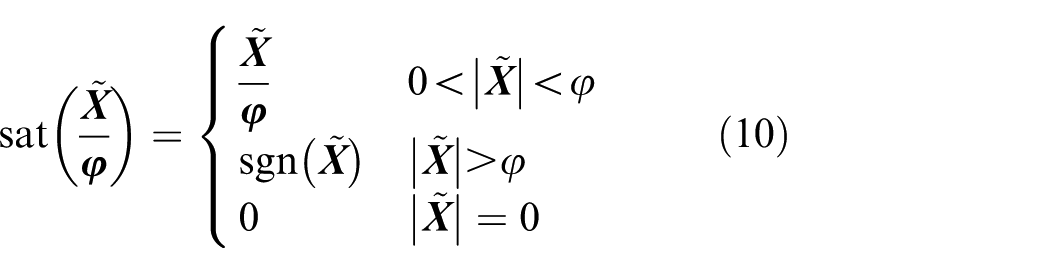
Establishment of vehicle model

In this article, we mainly discuss the distribution of the vehicle driving force, so the vehicle dynamics model needed to be simplified. As the vehicle suspension is simplified as a rigid suspension in our article, the roll angle and the pitch angle of the vehicle body are zero, the road surface is the soil, the influence of the air resistance is neglected, four wheels are used to drive, rear wheels are used to turn, the front and rear wheelbase are the same, the wheelbase is variable and the steering angle is simplified as being the same when the left rear wheel and right rear wheel are turning. Therefore, the vehicle can be simplified as a vehicle model with eight degrees of freedom, including longitudinal direction, side direction, the landscape orientation’s swing and the rear wheel’s turning and rotational degrees of freedom of the four wheels. A schematic diagram of the eight degrees of freedom of the vehicle model is shown in Figure 2. When the direction of the parameter is consistent with the direction of the graph, the sign is positive, and the sign is negative when the direction is the opposite.

Figure 2.

Vehicle dynamics model with eight degrees of freedom.

Longitudinal force balanced equation

$$m\left({\tilde{V}}_{\mathrm{x}}-\gamma ·V_{\mathrm{y}}\right)=F_{\mathrm{xfl}}+F_{\mathrm{xfr}}+\left(F_{\mathrm{xrl}}+F_{\mathrm{xrr}}\right)\cos \delta +\left(F_{\mathrm{yrl}}+F_{\mathrm{yrr}}\right)\sin \delta$$

(1)

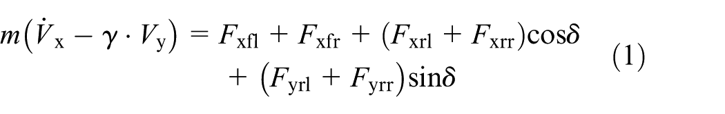
Lateral force balanced equation

$$m\left({\tilde{V}}_{\mathrm{y}}-\gamma ·V_{\mathrm{x}}\right)=F_{\mathrm{yfl}}+F_{\mathrm{yfr}}+\left(F_{\mathrm{yrl}}+F_{\mathrm{yrr}}\right)\cos \delta -\left(F_{\mathrm{xrl}}+F_{\mathrm{xrr}}\right)\sin \delta$$

(2)

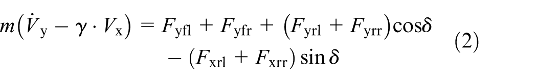
Balanced equation around Z axis

$$I_{\mathrm{z}}·\tilde{\gamma }=\left(F_{x\mathrm{f}r}-F_{\mathrm{xfl}}\right)\frac{W}{2}+\left(F_{\mathrm{yfl}}+F_{\mathrm{yfr}}\right)a+\left[\left(F_{\mathrm{xrl}}+F_{\mathrm{xrr}}\right)\sin \delta -\left(F_{\mathrm{yrl}}+F_{\mathrm{yrr}}\right)\cos \delta \right]b+\left[\left(F_{\mathrm{xrr}}-F_{\mathrm{xrl}}\right)\cos \delta +\left(F_{\mathrm{yrr}}-F_{\mathrm{yrl}}\right)\sin \delta \right]\frac{W}{2}$$

(3)

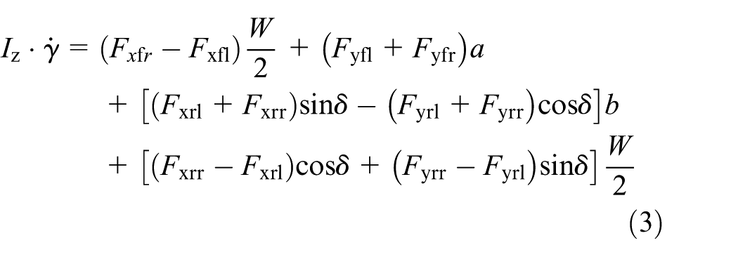
where δ is the rear wheel angle (rad); a and b are the distance between the front and rear axle to the centre of the vehicle (m); V_x and V_y are the longitudinal speed and lateral speed, respectively (m/s); $\gamma$ is the yaw rate (rad); L = a + b is the front and rear wheelbase (m); F_xi, F_yi and F_zi are the longitudinal force of the tyre, lateral force of the tyre and vertical force of the tyre, respectively; i is the left front wheel (f_l), right front wheel (f_r), left rear wheel (r_l) and right rear wheel (r_r); m is the weight of the whole vertical (kg); hg is the distance between the centroid and pavement (m); W is the distance between wheels (m); and I_z is the rotational inertia of the whole vertical rolling Z axle (kg m²).

Dynamics analysis of tyres

The vehicle’s longitudinal force, lateral force and swing moment are estimated by the slippage ratio, side slippage angle, adhesion coefficient and wheel supporting force. The support load of the wheel $(F_{\mathrm{zi}})$ can be calculated by Figure 2

$$\left[\begin{array}{c}{F}_{\mathrm{zfl}}\hfill \\ \multicolumn{1}{c}{F_{\mathrm{zfr}}}\\ \multicolumn{1}{c}{\begin{array}{c}{F}_{\mathrm{zrl}}\hfill \\ \multicolumn{1}{c}{F_{\mathrm{zrr}}}\end{array}}\end{array}\right]=\left[\begin{array}{c}\mathrm{mg}\frac{b}{2L}-m{\stackrel{·}{V}}_{\mathrm{x}}\frac{h_g}{2L}-\mathrm{mb}{\stackrel{·}{V}}_{\mathrm{y}}\frac{h_g}{L·W}\hfill \\ \multicolumn{1}{c}{\mathrm{mg}\frac{b}{2L}-m{\stackrel{·}{V}}_{\mathrm{x}}\frac{h_g}{2L}+\mathrm{mb}{\stackrel{·}{V}}_{\mathrm{y}}\frac{h_g}{L·W}}\\ \multicolumn{1}{c}{\mathrm{mg}\frac{a}{2L}+m{\stackrel{·}{V}}_{\mathrm{x}}\frac{h_g}{2L}-\mathrm{ma}{\stackrel{·}{V}}_{\mathrm{y}}\frac{h_g}{L·W}}\\ \multicolumn{1}{c}{\mathrm{mg}\frac{a}{2L}+m{\stackrel{·}{V}}_{\mathrm{x}}\frac{h_g}{2L}+\mathrm{ma}{\stackrel{·}{V}}_{\mathrm{y}}\frac{h_g}{L·W}}\end{array}\right]$$

(4)

The slip rate of the wheel in the process of accelerating can be calculated by the following formula

$$s=\frac{\omega r-\mathrm{Vvehicle}}{\omega r}$$

(5)

The distortion angle of the wheel can be calculated by the following formula

$$\left[\begin{array}{c}{\alpha }_{\mathrm{fl}}\hfill \\ \multicolumn{1}{c}{{\alpha }_{\mathrm{fr}}}\\ \multicolumn{1}{c}{\begin{array}{c}{\alpha }_{\mathrm{rl}}\hfill \\ \multicolumn{1}{c}{{\alpha }_{\mathrm{rr}}}\end{array}}\end{array}\right]=\left[\begin{array}{c}{\tan }^{-1}\left(\frac{V_{\mathrm{y}}+a·r}{V_{\mathrm{x}}-W·\frac{r}{2}}\right)\hfill \\ \multicolumn{1}{c}{{\tan }^{-1}\left(\frac{V_{\mathrm{y}}+a·r}{V_{\mathrm{x}}+W·\frac{r}{2}}\right)}\\ \multicolumn{1}{c}{\begin{array}{c}-\delta +{\tan }^{-1}\left(\frac{V_{\mathrm{y}}-b·r}{V_{\mathrm{x}}-W·\frac{r}{2}}\right)\hfill \\ \multicolumn{1}{c}{-\delta +{\tan }^{-1}\left(\frac{V_{\mathrm{y}}-b·r}{V_{\mathrm{x}}+W·\frac{r}{2}}\right)}\end{array}}\end{array}\right]$$

(6)

Observation instrumentation of tyre force

Observation instrument of tyre force commonly adopts variable sliding model structure, Kalman filter and other methods. In this article, the observation instrument designed by the variable sliding model structure is adopted, which has the advantage of a simple structure, robustness and so on. In the estimation of tyre force, the real-time performance and accuracy of the estimation should be considered, and the selection of the variable sliding model structure design can satisfy the needs of the design of the agricultural machinery.

According to the system state vector $\mathit{X}=({\omega }_{\mathrm{fl}},{\omega }_{\mathrm{fr}},{\omega }_{\mathrm{rl}},{\omega }_{\mathrm{rr}})$ , the observation vector of the system $\mathit{Z}=\mathit{X}$ and the dynamic analysis of Figure 2, the following equation can be obtained

$$\{\begin{array}{c}\stackrel{·}{\mathit{X}}={\mathit{A}}_{\mathrm{eq}}{\mathit{F}}_{\mathrm{eq}}+{\mathit{B}}_{\mathrm{eq}}{\mathit{T}}_{\mathrm{eq}}\hfill \\ \multicolumn{1}{c}{Z=X}\end{array}$$

(7)

where

$$\begin{array}{c}{\mathit{A}}_{\mathrm{eq}}=\left[\begin{array}{c}\begin{array}{ccc}-r/I_{\mathrm{z}}\hfill & 0\hfill & \begin{array}{cc}0\hfill & 0\hfill \end{array}\hfill \end{array}\hfill \\ \multicolumn{1}{c}{\begin{array}{ccc}0\hfill & -r/I_{\mathrm{z}}\hfill & \begin{array}{cc}0\hfill & 0\hfill \end{array}\hfill \end{array}}\\ \multicolumn{1}{c}{\begin{array}{c}\begin{array}{ccc}0\hfill & 0\hfill & \begin{array}{cc}-r/I_{\mathrm{z}}\hfill & 0\hfill \end{array}\hfill \end{array}\hfill \\ \multicolumn{1}{c}{\begin{array}{ccc}0\hfill & 0\hfill & \begin{array}{cc}0\hfill & -r/I_{\mathrm{z}}\hfill \end{array}\hfill \end{array}}\end{array}}\end{array}\right]\hfill \\ {\mathit{F}}_{\mathrm{eq}}={\left[\begin{array}{ccc}{F}_{\mathrm{xfl}}\hfill & F_{\mathrm{xfr}}\hfill & \begin{array}{cc}{F}_{\mathrm{xrl}}\hfill & F_{\mathrm{xrr}}\hfill \end{array}\hfill \end{array}\right]}^{\mathrm{T}}\hfill \\ {\mathit{B}}_{\mathrm{eq}}=\left[\begin{array}{ccc}1\hfill & 0\hfill & \begin{array}{cc}0\hfill & 0\hfill \end{array}\hfill \\ \multicolumn{1}{c}{0}& 1\hfill & \begin{array}{cc}0\hfill & 0\hfill \end{array}\hfill \\ \multicolumn{1}{c}{\begin{array}{c}0\hfill \\ \multicolumn{1}{c}{0}\end{array}}& \begin{array}{c}0\hfill \\ \multicolumn{1}{c}{0}\end{array}\hfill & \begin{array}{cc}\begin{array}{c}1\hfill \\ \multicolumn{1}{c}{0}\end{array}\hfill & \begin{array}{c}0\hfill \\ \multicolumn{1}{c}{1}\end{array}\hfill \end{array}\hfill \end{array}\right]\hfill \\ {\mathit{T}}_{\mathrm{eq}}={\left[\begin{array}{ccc}\frac{T_{\mathrm{fl}}}{I_{\mathrm{z}}}\hfill & \frac{T_{\mathrm{fr}}}{I_{\mathrm{z}}}\hfill & \begin{array}{cc}\frac{T_{\mathrm{rl}}}{I_{\mathrm{z}}}\hfill & \frac{T_{\mathrm{rr}}}{I_{\mathrm{z}}}\hfill \end{array}\hfill \end{array}\right]}^{\mathrm{T}}\hfill \end{array}$$

where T_ij is the driving moment of the wheel, and ij are defined as the left-front wheel (fl), the right-front wheel (fr), the left-rear wheel (rl) and the right-rear wheel (rr). To establish the state equation, design the sliding observation instrumentation as follows

$$\stackrel{·}{\hat{\mathit{X}}}={\mathit{B}}_{\mathrm{eq}}{\mathit{T}}_{\mathrm{eq}}+\mathit{h}(\tilde{\mathit{X}})$$

(8)

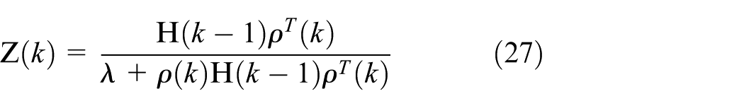
where $\tilde{\mathit{X}}$ is the error between observed and actual numbers, $\mathit{h}(\tilde{\mathit{X}})$ is the controlling parameter of the sliding model.

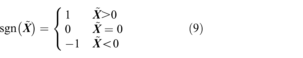
There are various choices for the controlling parameter of the sliding model. Due to the effect of forced switching and robustness of the sign function, the sign function sgn() is used as the controlling parameter of the sliding model in this article, namely, $\mathit{h}(\tilde{\mathit{X}})=\mathrm{sgn}(\tilde{\mathit{X}})$ . The controlling parameter of the sliding model can restrain the output, but it can also cause a shaking and make the observation effect be not ideal. Therefore, to avoid violent jitter of the estimation value, the boundary value is often used so that the estimation value can be stably close to the target value when the deviation is close to 0. However, solely using the sign function cannot eliminate the jitter of forced switching, so it is necessary to increase the approaching index to restrain the jitter. The approaching index can not only ensure the dynamic characteristics of the controlling process of the sliding model but also restrain high-frequency jitter. Therefore, after optimization, the sign function and the approaching index can effectively restrain the jitter. The expression of the sign function is as follows

$$\mathrm{sgn}\left(\tilde{\mathit{X}}\right)=\{\begin{array}{cc}1\hfill & \tilde{\mathit{X}}>0\hfill \\ \multicolumn{1}{c}{0}& \tilde{\mathit{X}}=0\hfill \\ \multicolumn{1}{c}{-1}& \tilde{\mathit{X}}<0\hfill \end{array}$$

(9)

The optimized boundary sign function is as follows

$$\mathrm{sat}\left(\frac{\tilde{\mathit{X}}}{\mathbf{\phi }}\right)=\{\begin{array}{cc}\frac{\tilde{\mathit{X}}}{\mathbf{\phi }}\hfill & 0<\left|\tilde{\mathit{X}}\right|<\phi \hfill \\ \multicolumn{1}{c}{\mathrm{sgn}\left(\tilde{\mathit{X}}\right)}& \left|\tilde{\mathit{X}}\right|>\phi \hfill \\ \multicolumn{1}{c}{0}& \left|\tilde{\mathit{X}}\right|=0\hfill \end{array}$$

(10)

where $\mathbf{\phi }$ is the thickness of the boundary. The expression of the controlling parameter of the sliding model is as follows

$$\mathit{h}\left(\tilde{\mathit{X}}\right)=\mathit{k}·\tilde{\mathit{X}}+\mathrm{sat}\left(\frac{\tilde{\mathit{X}}}{\mathbf{\phi }}\right)$$

(11)

where k is the parameter of the approaching index. The error of the observation instrument is

$$\stackrel{·}{\stackrel{~}{\mathit{X}}}={\mathit{A}}_{\mathrm{eq}}{\mathit{F}}_{\mathrm{eq}}-[\mathit{k}·\tilde{\mathit{X}}+\mathrm{sat}\left(\frac{\tilde{\mathit{X}}}{\mathbf{\phi }}\right)]$$

(12)

As the input and output make up the actual vehicle model, the data-in and the state are all bounded values; in other words, the observed value is bounded. To verify the stability of the system, the Lyapunov function is established

$$V_i=\frac{1}{2}{\tilde{x}}_i^2(i=\mathrm{fl},\mathrm{fr},\mathrm{rl},\mathrm{rr})$$

(13)

The derivation of the Lyapunov function is as follows

$$\stackrel{·}{\mathit{V}}={\tilde{\mathit{X}}}^{\mathrm{T}}\stackrel{·}{\stackrel{~}{\mathit{X}}}={\tilde{\mathit{X}}}^{\mathrm{T}}\{{\mathit{A}}_{\mathrm{eq}}{\mathit{F}}_{\mathrm{eq}}-[\mathit{k}·\tilde{\mathit{X}}+\mathrm{sat}\left(\frac{\tilde{\mathit{X}}}{\mathbf{\phi }}\right)]\}$$

(14)

It can be seen that the error of the system is stable when the number k is infinite $\stackrel{·}{\mathit{V}}<0$ and the error approaches zero in limited time. The error $(\stackrel{·}{\stackrel{~}{\mathit{X}}}=0)$ is taken into formula (12), and the following formula can be obtained

$${\mathit{A}}_{\mathrm{eq}}{\mathit{F}}_{\mathrm{eq}}=\mathit{k}·\tilde{\mathit{X}}+\mathrm{sat}\left(\frac{\tilde{\mathit{X}}}{\mathbf{\phi }}\right)$$

(15)

Transform formula (15) and the observation value can be obtained as shown in the following

$$\widehat{{\mathit{F}}_{\mathrm{eq}}}={{\mathit{A}}_{\mathrm{eq}}}^{-1}[\mathit{k}·\tilde{\mathit{X}}+\mathrm{sat}\left(\frac{\tilde{\mathit{X}}}{\mathbf{\phi }}\right)]$$

(16)

Estimation of adhesion coefficient

Estimation of recursive least square method

Based on the observation of the tyre force, the existing tyre model can be used to estimate the parameters of the recursive least square method and the adhesion coefficient of the road surface can be obtained. At present, the tyre model is generally used as a magic formula; however, the parameters of the magic formula are more complex, and the calculation amount of the magic formula is large, so a relatively simple brush tyre model is adopted, and it is mainly based on the assumption of the elastic tread and the rigid body. The characteristic of the relatively simple brush tyre model is that it is assumed that the elasticity of the tyre is completely concentrated on the surface of the brush deformation. The longitudinal force expression of the brush tyre model is as follows

$$F_{\mathrm{x}}=\frac{C_{\mathrm{x}}\left(\frac{k}{1+k}\right)}{f}·F_{\mathrm{t}}$$

(17)

where

$$\begin{array}{c}{F}_{\mathrm{t}}=\{\begin{array}{cc}\begin{array}{c}f-\frac{1}{3\mu F_{\mathrm{z}}}{f}^2+\frac{1}{27{\mu }^2{F}_z^2}{f}^3\hfill \\ \multicolumn{1}{c}{\mu F_{\mathrm{z}}}\end{array}\hfill & \begin{array}{c}f<3\mu F_{\mathrm{z}}\hfill \end{array}\hfill \end{array}\hfill \\ f=\sqrt{C_{\mathrm{x}}^2{\left(\frac{k}{1+k}\right)}^2+C_{\mathrm{\alpha }}^2{\left(\frac{\tan \alpha }{1+k}\right)}^2}\hfill \end{array}$$

where $C_{\mathrm{\alpha }}$ is the lateral stiffness of the tyre, $C_{\mathrm{x}}$ is the longitudinal stiffness of the tyre and $\mu$ is the adhesion coefficient of the road surface.

The three parameters of the brush model need to be estimated, and the tyre stiffness can be seen as a fixed value in a test; thus, the tyre model has only one parameter to be identified, which is the adhesion coefficient. The adhesion coefficient can be estimated by recursive least squares algorithm.

Because the brush tyre model is segmented, it needs to be linearized. The brush model can be changed to the following formula

$$y\left(k\right)=f(k,\mu \left(k\right))+\epsilon$$

(18)

where $\mathit{y}=[F_{\mathrm{xfl}},F_{\mathrm{xfr}},F_{\mathrm{xrl}},F_{\mathrm{xrr}}]$ is estimated by the observation instrumentation of the tyre force, $f(k,\mu (k))$ is a simplified expression for a brush model and $\epsilon$ is defined so that noise is introduced into the observation.

To estimate the adhesion coefficient, formula (18) should be calculated approximately as follows

$$y\left(k\right)\approx f(k,\hat{\mu }(k-1))+\rho \left(k\right)(\hat{\mu }\left(k\right)-\hat{\mu }(k-1))$$

(19)

where

$$\rho \left(k\right)=\frac{\partial f(k,\mu )}{\partial \mu }|\begin{array}{c}\multicolumn{1}{c}{\mu =\hat{\mu }(k-1)}\end{array}$$

(20)

Variable $h(k)$ is set

$$h\left(k\right)=y\left(k\right)+\rho \left(k\right)\hat{\mu }(k-1)-f(k,\hat{\mu }(k-1))$$

(21)

The following formula is obtained

$$h\left(k\right)\approx \rho \left(k\right)\hat{\mu }\left(k\right)$$

(22)

The value function of recursive least squares is set

$$J(\hat{\mu },k)=\sum _{i=1}^k{\lambda }^{k-i}(h\left(i\right)-\rho \left(i\right)\hat{\mu }{)}^2$$

(23)

where $\lambda$ is the factor of forgetting. Taking a derivative with respect to formula (23) obtains a new formula $\hat{\mu }$ , which is shown as follows

$$\hat{\mu }\left(k\right)={\left(\sum _{i=1}^k{\rho }^T\left(i\right){\lambda }^{k-i}\rho \left(i\right)\right)}^{-1}\sum _{i=1}^k{\rho }^T\left(i\right){\lambda }^{k-i}h\left(i\right)$$

(24)

The covariance matrix is used as $\mathrm{H}(k)$ and is shown as follows

$$\mathrm{H}\left(k\right)={\left(\sum _{i=1}^k{\rho }^T\left(i\right){\lambda }^{k-i}\rho \left(i\right)\right)}^{-1}$$

(25)

The following formula is obtained by Sherman–Morrison recursive calculation

$$\mathrm{H}\left(k\right)=\frac{1}{\lambda }[\mathrm{H}(k-1)-\frac{\mathrm{H}(k-1){\rho }^T\left(k\right)\rho \left(k\right)\mathrm{H}(k-1)}{\lambda +\rho \left(k\right)\mathrm{H}(k-1){\rho }^T\left(k\right)}]$$

(26)

The recursive least squares iterative formula is obtained, which is shown as follows

$$\mathrm{Z}\left(k\right)=\frac{\mathrm{H}(k-1){\rho }^T\left(k\right)}{\lambda +\rho \left(k\right)\mathrm{H}(k-1){\rho }^T\left(k\right)}$$

(27)

$$\hat{\mu }\left(k\right)=\hat{\mu }(k-1)+\mathrm{Z}\left(k\right)·(h\left(k\right)-\rho \left(k\right)\hat{\mu }(k-1))$$

(28)

$$\mathrm{H}\left(k\right)=\frac{1-\mathrm{Z}\left(k\right)\rho \left(k\right)}{\lambda }\mathrm{H}(k-1)$$

(29)

Simplification of tyre model

In practice, the vehicle cannot directly measure the pavement in real time. Currently, the magic formula is generally used to describe the mechanical properties of the tyre, but because of its complex mathematical form, computer simulation is generally used. In this article, to establish a real-time control system, the tyre model is simplified, and its accuracy is also required. By reading the literature, a simplified tyre model formula is obtained that has fewer parameters and is relatively accurate. Its form is as follows

$$\mu \left(\mathrm{S}\right)=\frac{2{\mu }_{\mathrm{p}}{S}_{\mathrm{p}}S}{{S_{\mathrm{p}}}^2+S^2}$$

(30)

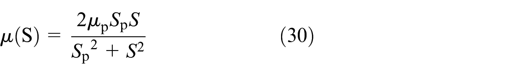
where S is the slip rate, ${\mu }_{\mathrm{p}}$ is the peak adhesion coefficient and $S_{\mathrm{p}}$ is the slip rate corresponding to the peak adhesion coefficient (Figure 3).

Figure 3.

Relationship between slip ration of simplified model and adhesion coefficient.

From the data obtained, the adhesion coefficients ${\mu }_1\mathrm{and}{\mu }_2$ and the slip rates $s_1\mathrm{and}{s}_2$ were collected and utilized. If A is defined as $S_{\mathrm{p}}^2$ and B is defined as $2{\mu }_{\mathrm{p}}{S}_{\mathrm{p}}$ , then the following formula is obtained by changing the form of formula (30)

$$\{\begin{array}{c}A=\frac{\frac{{\mu }_1}{{\mu }_2}{s}_1-s_2}{s_1-\frac{{\mu }_1}{{\mu }_2}{s}_2}{s}_1{s}_2\hfill \\ B=\frac{{s_1}^2-{s_2}^2}{\frac{{\mu }_1}{s_1}-\frac{{\mu }_2}{s_2}}\hfill \end{array}$$

(31)

The identifier technique of road surface conditions of vehicle driving

Parameter setting of vehicle running status

The setting of vehicle status parameters can contribute to understanding conditions of vehicles and can use the threshold to select different control systems.

The setting of vehicle status parameters mainly includes vehicles starting flag, reaching the target speed flag, driving control flag and road surface separation flag (Table 1).

Table 1.

Set flag.

Vehicle flag bit variable	Flag bit name	Remarks
Start	Vehicle starting flag	Whether is in starting stage or not  If Start = 1, it is in starting stage  If Start = 0, it is not in starting stage
DriveOn	Driving control flag	Whether drive control begins  If DriveOn = 1, drive control begins  If DriveOn = 0, drive control does not begin
RoadDif	Separation road surface flag bit	Whether is road surface separation or not  If RoadDif = 1, it is separation road surface  If RoadDif = 0, it is road uniform surface
Slipfl	Target speed of the left front wheel flag	Whether the wheels reach target speed  If X = 1, the wheels reach target speed  If X = 0, the wheels cannot reach target speed X represents parameters of four wheels flag
Slipfr	Target speed of the right front wheel flag
Sliprl	Target speed of the left rear wheel flag
Sliprr	Target speed of the right rear wheel flag

The identifier method of detached state of vehicle driving road surface

Road surface separation flag is used to judge whether the vehicle is driving on working condition that the difference of adhesion coefficient of left and right pavement is in a certain range. In this article, only accelerating straight driving is considered, so only c the difference of adhesion coefficient of the left and right side of the wheel is considered within a certain range.

When the absolute value of the difference between the left front wheel adhesion coefficient µ_fl and the right front wheel adhesion coefficient µ_fr is greater than the set value, the delay judgement is carried out to eliminate the road interference. After a certain number of times, the delay judgement still holds, the RoadDif is set as 1 and the vehicle is running on the separation road surface. Similarly, the left rear wheel adhesion coefficient µ_rl and the right rear wheel adhesion coefficient µ_rr are also determined according to the principle (Figure 4).

Figure 4.

The mart of split cohesion coefficient road.

Control strategy of high-clearance electric driving vehicle

Due to the driving forces of the four wheels of high-clearance electric driving vehicles being different from each other, there are various modes of driving control. The driving force of each wheel can be controlled separately, and the driving control mainly includes the anti-slip driving control and the anti-deviate moment control.

Control block diagram of vehicle driving

In the agricultural environment, especially the intertillage stage, high ground clearance vehicle runs in plant roots, and the adhesion coefficient of the ground is constantly changing, and there may be significant differences in adhesion coefficients between the lines. The adhesion coefficient of plant roots cannot be obtained by means of observation, so it is necessary to adjust the control strategy according to the driving state. It mainly includes the driving intention of the driver, the calculation of the driving state of the vehicle, whether the road is uniform or not, driving on high and low adhesion road surface, the working condition and the coordinated control of the straight line (Figure 5).

Figure 5.

Control flowchart.

Control theory of the slip rate

Agricultural machinery, especially machinery for plant protection, are working for intertillage. As the crops grow, the wheels can only drive through the crop inter-row. In addition, the distance between wheels is larger, and soil change is more obvious; therefore, a good ability to drive straight is needed to keep from crushing the crop. With traditional machinery, due to the presence of the differential mechanism, the driving force of other wheels will be significantly reduced when a wheel completely slips. Although it can be guaranteed that traditional machinery will drive straight to a certain degree, the overall efficiency of the vehicle will be reduced. For four-wheel independent drive vehicles, the other side is not affected while one side of the vehicle slips. The power and efficiency of the four-wheel independent drive vehicles are enhanced, but the lateral stability of the vehicle is reduced, such that the vehicles may not drive straight. To keep the vehicles driving straight, the driving force of the left and right driving wheels of the vehicle must be controlled, which requires consideration of the efficiency and lateral stability. In this article, the design project of the sliding rate comes from sliding mode structure control and incremental proportional–integral (PI) control, as shown in Figure 6.

Figure 6.

Sketch map of high ground clearance vehicle.

Driving control based on the variable sliding mode structure

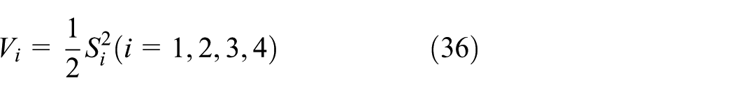
The parameters of the soil are different when the vehicles drive in different environments, so it is difficult to accurately obtain the soil parameters, which can only be predicted by the existing parameters at home. Sliding mode control can effectively solve uncertain nonlinear systems, which has the advantages of robustness and fast response.

Constructing the state equation of the control system and taking the derivative of equation (30) are as follows

$${\stackrel{·}{s}}_i=\frac{r{(1-s_i)}^2(T_i-T_{\mathrm{R}i})}{\mathrm{Jv}}-\frac{(1-s_i)\sum _{i=1}^4{F}_{\mathrm{T}i}}{\mathrm{Mv}}(i=1,2,3,4)$$

(32)

The following equation is obtained by rewriting equation (32)

$$\stackrel{·}{\mathit{s}}=\mathit{h}(\mathit{s},v)+g(\mathit{s},v)\mathit{u}$$

(33)

where

$$\begin{array}{c}\mathit{s}=[\begin{array}{cccc}{s}_1\hfill & s_2\hfill & s_3\hfill & s_4\hfill \end{array}{]}^{\mathrm{T}}\hfill \\ \mathit{u}=[\begin{array}{cccc}{T}_1\hfill & T_2\hfill & T_3\hfill & T_4\hfill \end{array}{]}^{\mathrm{T}}\hfill \\ \mathit{h}(\mathit{s},v)=[\begin{array}{cccc}{h}_1(s,v)\hfill & h_2(s,v)\hfill & h_3(s,v)\hfill & h_4(s,v)\hfill \end{array}{]}^{\mathrm{T}}\hfill \\ \mathit{g}(\mathit{s},v)=\mathrm{diag}\left[\begin{array}{cccc}{g}_1(s,v)\hfill & g_2(s,v)\hfill & g_3(s,v)\hfill & g_4(s,v)\hfill \end{array}\right]\hfill \\ h_i(\mathit{s},v)=-\frac{r{(1-s_i)}^2{T}_{\mathrm{R}i}}{\mathrm{Jv}}-\frac{(1-s_i)\sum _{i=1}^4{F}_{\mathrm{T}i}}{\mathrm{Mv}}\hfill \\ g_i(\mathit{s},v)=\frac{r{(1-{\mathit{s}}_i)}^2}{J\mathit{v}}i=1,2,3,4\hfill \end{array}$$

We define the sliding surface as $\mathit{S}=\mathit{s}-{\mathit{s}}_{\mathrm{q}}$ , and ${\mathit{s}}_{\mathrm{q}}$ is the desired slip rate vector, set by us. Thus, $\stackrel{·}{S}=\stackrel{·}{s}=h(s,v)+g(s,v)$ , and the approaching law of the sliding model is defined as

$$\stackrel{·}{\mathit{S}}=-\mathbf{\epsilon }\mathrm{sgn}\mathbf{\left(}\mathit{S}\mathbf{\right)}$$

(34)

where $\mathbf{\epsilon }\mathbf{=}\mathbf{[}\begin{array}{cccc}{\mathbf{\epsilon }}_1\hfill & {\mathbf{\epsilon }}_2\hfill & {\mathbf{\epsilon }}_3\hfill & {\mathbf{\epsilon }}_4\hfill \end{array}{\mathbf{]}}^{\mathrm{T}}$ and ${\epsilon }_i>0$ (i = 1, 2, 3, 3), and $\mathrm{sgn}(\mathit{x})$ is the sign function, the definition of which is

$$\mathrm{sgn}\left(\mathbf{x}\right)=\{\begin{array}{c}1\hfill \\ \multicolumn{1}{c}{0}\\ \multicolumn{1}{c}{-1}\end{array}\begin{array}{c}\mathbf{x}>0\hfill \\ \multicolumn{1}{c}{\mathbf{x}=0}\\ \multicolumn{1}{c}{\mathbf{x}<0}\end{array}$$

(35)

To ensure the stability of the sliding control, namely, to satisfy $S_i{\stackrel{·}{S}}_i<0$ , Lyapunov is constructed and shown as follows

$$V_i=\frac{1}{2}{S}_i^2(i=1,2,3,4)$$

(36)

As ${\stackrel{·}{V}}_i=S_i{\stackrel{·}{S}}_i=-{\epsilon }_i\mathrm{sgn}(S_i)·S_i=-{\epsilon }_i\left|S_i\right|$ and $S$ is close to zero, the system is stable, namely, ${\stackrel{·}{V}}_i<0$ . The relationship between the control variables u and the input s and v is calculated

$$T_i=T_{\mathrm{R}i}+\frac{J\sum _{i=1}^4{F}_{\mathrm{T}i}}{\mathrm{Mr}(1-s_i)}-\frac{\mathrm{Jv}}{r{(1-s_i)}^2}{\epsilon }_i\mathrm{sgn}\left(S_i\right)(i=1,2,3,4)$$

(37)

$\mathit{u}$ is divided into two parts, which are the balance driving moment ${\mathit{T}}_{\mathrm{eq}}$ and non-balance driving moment ${\mathit{T}}_{\mathrm{ueq}}$ , and they can be indicated as

$$\mathit{u}={\mathit{T}}_{\mathrm{eq}}-{\mathit{T}}_{\mathrm{ueq}}$$

(38)

where

$$\begin{array}{c}\mathit{u}=[T_1{T}_2{T}_3{T}_4{]}^{\mathrm{T}}\hfill \\ {\mathit{T}}_{\mathrm{eq}}=[T_{\mathrm{eq}1}{T}_{\mathrm{eq}2}{T}_{\mathrm{eq}3}{T}_{\mathrm{eq}4}{]}^{\mathrm{T}}\hfill \\ {\mathit{T}}_{\mathrm{ueq}}=[T_{\mathrm{ueq}1}{T}_{\mathrm{ueq}2}{T}_{\mathrm{ueq}3}{T}_{\mathrm{ueq}4}{]}^{\mathrm{T}}\hfill \end{array}$$

(38)

To eliminate the jitter of the variable sliding mode structure, ${\mathit{T}}_{\mathrm{ueq}}=\mathrm{Jv}/r(1-\mathit{s}{)}^2\mathbf{\epsilon }\mathrm{sat}\mathbf{(}\mathit{S}\mathbf{/}\mathbf{\phi }\mathbf{)}$ is set, and

$$\mathrm{sat}\left(\frac{\mathit{S}}{\mathbf{\phi }}\right)=\{\begin{array}{cc}\frac{\mathit{S}}{\mathbf{\phi }}\hfill & 0<\left|\mathit{S}\right|<\phi \hfill \\ \multicolumn{1}{c}{\mathrm{sgn}\left(\mathit{S}\right)}& \left|\mathit{S}\right|>\phi \hfill \\ \multicolumn{1}{c}{0}& \left|\mathit{S}\right|=0\hfill \end{array}$$

(39)

where $\mathbf{\phi }$ is the thickness of the boundary layer.

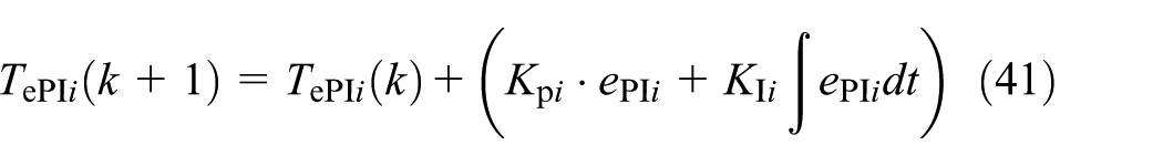
Driving control based on incremental PI control

As shown in Figure 7, with the increase in the slip rate, the longitudinal and lateral adhesion coefficients of the road surface are changing to make the vehicle have good longitudinal adhesion and not lose too much lateral force; thus, the slip rate of the tyres needs to be maintained to within a certain range.

Figure 7.

Relationship between slip ratio and adhesion coefficient.

Longitudinal force $F_{\mathrm{x}}=F_{\mathrm{z}}{\mu }_{\mathrm{x}}$ and lateral force $F_{\mathrm{y}}=F_{\mathrm{z}}{\mu }_{\mathrm{y}}$ . In this article, as the support force of each wheel is unchanged, the change relationship between the change of the longitudinal force and lateral force and slip rate is shown in Figure 7. According to the second chapter, the following is concluded

$$J\stackrel{·}{\omega }=T-F_{\mathrm{x}}*R$$

(40)

When the vehicle is in different roads, it is required to ensure that the vehicle’s driving force of the left and right sides of the wheel have the same direction and the same size, which makes the vehicle run at a certain acceleration in a straight line.

The front and rear wheels are controlled by incremental PI control, and the appropriate target slip ratio $s_{\mathrm{e}i}$ is selected by the test. If $e_{\mathrm{PI}i}=s_{\mathrm{e}i}-s_i$ , then the incremental PI control is expressed as

$$T_{\mathrm{ePI}i}(k+1)=T_{\mathrm{ePI}i}\left(k\right)+(K_{\mathrm{p}i}·e_{\mathrm{PI}i}+K_{\mathrm{I}i}\int e_{\mathrm{PI}i}\mathrm{dt})$$

(41)

where $K_{\mathrm{p}i}\mathrm{and}{K}_{\mathrm{I}i}$ is the control parameter of the incremental PI control. I represents the left front wheel (fl), right front wheel (fr), left rear wheel (rl) and right rear wheel (rr).

Driving force ratio of front and rear axle

The difference between the four-wheel independent driving vehicle and the traditional mechanical vehicle is that the variation of the driving force ratio of the independent driving vehicle can be controlled at any time, and it can be adjusted according to the specific driving state of the vehicle. In this article, the theory of the tyre friction circle is adopted and can guarantee the longitudinal and lateral stability of the vehicle

$$F_{\mathrm{x}}^2+F_{\mathrm{y}}^2={(\mu ·F_{\mathrm{z}})}^2$$

(42)

Analysing the same side of the wheel, it can be seen as a model of the two-wheel vehicle, as shown in Figure 8.

Figure 8.

Two-wheel simplified model.

The offset of the wheel load can be calculated when the wheel is accelerating, and it is indicated as $\Delta w$

$$\Delta w=(F_{\mathrm{xf}}+F_{\mathrm{xr}})·\frac{h}{L}$$

(43)

where h is the centre of the vehicle height, and L is the front and rear wheelbase. Therefore, the distribution relationship of lateral force between the front and rear wheels is

$$\{\begin{array}{c}{F}_{\mathrm{yf}}=m·a_{\mathrm{y}}·\frac{b}{L}\hfill \\ \multicolumn{1}{c}{F_{\mathrm{yr}}=m·a_{\mathrm{y}}·\frac{a}{L}}\end{array}$$

(44)

The front wheel friction circle equation is

$$F_{\mathrm{xf}}^2+F_{\mathrm{yf}}^2={(\mu ·(F_{\mathrm{zf}}-\Delta w))}^2$$

(45)

The rear wheel friction circle equation is

$$F_{\mathrm{xr}}^2+F_{\mathrm{yr}}^2={(\mu ·(F_{\mathrm{zr}}+\Delta w))}^2$$

(46)

The following formula can be obtained by substituting formula (43) into formulas (44)–(46)

$$F_{\mathrm{xf}}^2+{(m·a_{\mathrm{y}}·\frac{b}{L})}^2={[\mu ·(F_{\mathrm{zf}}-(F_{\mathrm{xf}}+F_{\mathrm{xr}})·\frac{h}{L})]}^2$$

(47)

$$F_{\mathrm{xr}}^2+{(m·a_{\mathrm{y}}·\frac{a}{L})}^2={[\mu ·(F_{\mathrm{zr}}+(F_{\mathrm{xf}}+F_{\mathrm{xr}})·\frac{h}{L})]}^2$$

(48)

where $\mu$ can be estimated by the algorithm in the second chapter, which is known here. The ideal allocation relationship between the front and rear wheels can be obtained

$$C_{\mathrm{r}}=\frac{F_{\mathrm{xr}}}{F_{\mathrm{xr}}+F_{\mathrm{xf}}}$$

(49)

where $C_{\mathrm{r}}$ is the proportion of the rear wheel.

In formula (49), the unknown amount can be eliminated, and the relationship of the proportion of the rear wheel, longitudinal acceleration and pavement’s adhesion coefficient can be obtained by the simultaneous relationship from formulas (47)–(49)

$$C_{\mathrm{r}}=f(a_{\mathrm{x}},\mu )$$

(50)

Road driving conditions and control

The driving conditions of agricultural vehicles in the field are divided into two categories: uniform and separate road pavement; the uniform road can be divided into high-adhesion and low-adhesion road pavement. The linear driving conditions comprise five types: driving straight on a uniform road (single attachment), driving straight from high- to low-adhesion road attachment on a uniform road, driving straight from low- to high-adhesion road attachment on a uniform road, driving straight on a separated road and driving straight on a mixed complex road.

Starting stage

We first read the gear set by the current operator and used the pre-set driving force for driving. We put the Start position at 1, which indicates that the vehicle has just started, and we did not take other control measures. When the GPS feedback vehicle speed reached the specified speed, the Start was set to 0, which indicated that the vehicle had exited the start stage. After the ending start, the state of RoadDif flag was set. When the RoadDif flag was set to 0, it indicated that the vehicle was driving on a uniform road; otherwise, the vehicle was driving on a separate road.

Straight line acceleration driving on uniform road

When the RoadDif flag was set to 0, the Start was set to 0 and the DriveOn was set to 1, then we could judge that the vehicle was driving on a uniform road, set the target slip rate to 15%, and begin to call the sliding mode variable structure to control the slip rate or start the incremental PI to control the slip rate.

Straight line acceleration driving on separated Road

When the RoadDif flag was set to 1, the Start was set to 0 and the DriveOn was set to 1, then we could judge that the vehicle was driving on a separated road. We then set the target of adhesion coefficient to 0.2 and began to call the sliding mode variable structure to control the slip rate or start the incremental PI to control the slip rate.

Road test and results

According to the attached condition of the road, uniform pavement and separate pavement were selected as the test pavement. The test was carried out by not adopting the control strategy and adopting the variable sliding mode control strategy.

Parameter adjustment test

The parameters of adjustment increment PI value as follows. The values of the loop gain K_pfl, K_prl, K_pfr and K_prr are 20, 20, 10 and 10, respectively, and the values of the integration time K_Ifl, K_Irl, K_Ifr and K_Irr are 1.0, 1.0, 1.0 and 1.0 min, respectively. Figure 9 is obtained by the increment PI control.

Figure 9.

Wheel slip ratio of incremental PI control.

To better adjust the parameters, in this article, the suspension experiment method was first adopted, and the vehicle speed was set at 0.5 m/s, which was a constant value. In addition, the target slip rate is 0.08. The control parameters of the sliding mode control were adjusted

$$\begin{array}{c}\mathbf{\epsilon }\mathbf{=}\mathbf{[}0\mathbf{.}05\mathbf{,}0\mathbf{.}05\mathbf{,}0\mathbf{.}05\mathbf{,}0\mathbf{.}05\mathbf{]}\hfill \\ \mathbf{\phi }\mathbf{=}\mathbf{[}0\mathbf{.}001\mathbf{,}0\mathbf{.}001\mathbf{,}0\mathbf{.}001\mathbf{,}0\mathbf{.}001\mathbf{]}\hfill \end{array}$$

(50)

The control results are shown in Figure 10.

Figure 10.

Wheel slip ratio of sliding model control.

It can be seen from the experiment that the sliding mode control algorithm can control the slip ratio very well in the real vehicle test, which verified the feasibility of the control theory.

Uniform pavement test

In the test, the open land of the agricultural machinery test assay station of Jiangsu province was selected as the test site. The site can be divided into soil road covered with hay and mud road covered with new growing grass, which can be seen in Figure 11. Because the length of the site is approximately 30 m and the points collected at each test of the vehicles is approximately 50, many experiments are needed to verify the conclusion.

Figure 11.

Test site.

The influence of external interference on the system can be reflected by the road test data of slip ration without the control strategy. Figure 12 is the vehicle speed change curve without control strategy. The slip ration of the vehicle without any control strategy under this speed curve is shown in Figure 12.

Figure 12.

Speed of no control strategy.

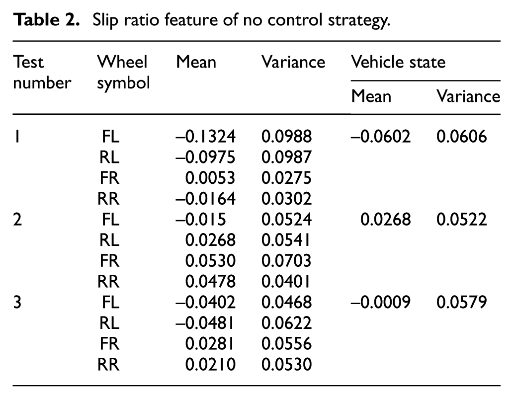
As can be seen from Figure 13, slip rate have larger fluctuation under the condition of a given input torque free walk. In order to better describe the wheel slip rate, the data of volatility are characterized using mean and variance of the torque stability slip rate, as shown in Table 2.

Table 2.

Slip ratio feature of no control strategy.

Test number	Wheel symbol	Mean	Variance	Vehicle state
				Mean	Variance
1	FL	–0.1324	0.0988	–0.0602	0.0606
	RL	–0.0975	0.0987
	FR	0.0053	0.0275
	RR	–0.0164	0.0302
2	FL	–0.015	0.0524	0.0268	0.0522
	RL	0.0268	0.0541
	FR	0.0530	0.0703
	RR	0.0478	0.0401
3	FL	–0.0402	0.0468	–0.0009	0.0579
	RL	–0.0481	0.0622
	FR	0.0281	0.0556
	RR	0.0210	0.0530

Figure 13.

Slip ratio of no control strategy.

The influence of external disturbance on the system is shown in Table 2. The slip ration of the wheel has changed greatly when travelling freely, and there is no guarantee that the slip ration of the four wheels is basically kept in a range.

Road test based on sliding mode variable structure control

It is known from previous studies that the optimal slip rate is 5.8%–8.7% in dry land. According to the data collected by the free walk, the estimated value $\mu$ of the adhesion coefficient of the road surface can be obtained using an adhesion coefficient estimation model to estimate and analyse, which is approximately 0.3, and the S is approximately 0.08. Because the optimum slip ratio of the road surface is 0.08, the selected target slip ratio selected is 0.08.

As seen from Figure 14, at 5 s, the vehicle speed exceeds 1 m/s, and the position of the Start mark is at 0; then, it can be seen from Figure 15 that the slip rate of the four wheels is similar, so the RoadDif is set to 0, the slippage of the four wheels is more than 0–0.2 from the range set before, so the DriveOn is set at 1 at 5 s, the vehicle begins to enter the automatic control mode, and the sliding mode variable structure control is executed.

Figure 14.

Speed of sliding model strategy for the vehicle.

Figure 15.

Slip ration of the incremental PI control strategy.

At 3 s, Figure 16 shows the slip ration of four wheels is similar, so RoadDif is set to 0, the slip rate of the four wheels exceeds the set 0–0.2 range. Thus, at 3 s, DriveOn is set to 1, the vehicle began to enter the automatic control mode and incremental PI control starts to perform.

Figure 16.

Slip ration of incremental PI strategy for vehicle.

The Gauss projection coordinates X: 159778, Y: 3557680 of the entrance of assay station were used as the origin of the new coordinate system, and the vehicle running track line can be obtained, as shown in Figure 17. The linear correlation coefficient is 0.9998 using linear regression calculation, so it is considered that the vehicle is driving straight.

Figure 17.

XY coordinates of sliding mode strategy for vehicle on uniform pavement.

To better describe the current sliding rate of the wheel, three groups of tests were randomly selected, and the volatility of the data is characterized using the mean and variance of the slip rate after control stability, as shown in Table 3.

Table 3.

Slip ratio feature of sliding model strategy.

Test serial number	Wheel symbol	Mean value	Variance	Vehicle state
				Mean value	Variance
1	FL	0.0577	0.0212	0.0722	0.0204
	RL	0.0554	0.0242
	FR	0.0458	0.0205
	RR	0.1299	0.0110
2	FL	0.0480	0.0248	0.0620	0.0198
	RL	0.0555	0.0210
	FR	0.0768	0.0139
	RR	0.0679	0.0189
3	FL	0.0836	0.0113	0.0774	0.0164
	RL	0.0487	0.0246
	FR	0.0975	0.0167
	RR	0.0801	0.0109

It can be seen from Table 3 that the slip rate of each wheel is close to 0.08, and compared to the wheels that had not taken the strategy, its control is relatively stable. Because of the difference in the road surface, the wheel control degree is different. According to the test, it is known that the basic stability degree is controlled to within 1 s.

It can be seen from the test programme above that the slip rate controlled by sliding mode is closer to the target value.

Separated pavement test

The main characteristic of high-clearance vehicles is the wide spaced work, and the road environment changes greatly; thus, the driving situation of separated road needs to be studied. The peak adhesion coefficient of the left and right side of the pavement and the corresponding optimal slip rate of the separate road surfaces are different. However, if a vehicle is required to travel in a straight line, then it is necessary to ensure that the adhesion coefficients of the wheels are the same (Figure 18).

Figure 18.

Test of isolated road.

Road test based on sliding mode variable structure control

According to the pavement parameters obtained from the test, the best slip can be calculated when the right wheel is on the soil surface, and the best slip rate is 0.08. The adhesion coefficient is 0.3. As shown in Figure 19, the slip rate of the wheel is 0.03, which is required when the vehicles are driving on the cement pavement. When the slip rate of the right wheel is set to 0.08 and the slip rate of the left wheel is set to 0.03, then Figure 19 can be obtained.

Figure 19.

Slip ratio of sliding model strategy.

The incremental PI control algorithm is used to control the vehicle, and the basic parameters refer to the setting of the previous section. The slip ration is shown in Figure 20.

Figure 20.

Slip ratio of incremental PI strategy for vehicle.

The adhesion coefficients of wheels can be obtained using the estimating method, as shown in Figure 21.

Figure 21.

Adhesion coefficient of sliding model strategy.

It is clear that if the adhesion coefficient is basically consistent, then the acceleration performance of the left and right wheels can be the same, and the vehicle can be driven straight. According to the XY axis collected by the GPS, Figure 22 can be drawn.

Figure 22.

XY coordinates of sliding mode strategy for vehicle on separated pavement.

Test summary

In this section, the peak adhesion coefficient and the corresponding slip rate of the left and right sides of the split cohesion coefficient road are mainly introduced. The required slip rates of the left and right sides are calculated to be 0.03 and 0.08, respectively. Two control algorithms are used to control the split cohesion coefficient road, and the results showed that the sliding mode variable structure control strategy is more suitable for the control of the split cohesion coefficient road.

In this chapter, the control parameters of the vehicle were adjusted by the suspension test method, and acceptable results were obtained, which indicated that the algorithm is effective. Then, three kinds of control strategies were used to test the uniform pavement and the separate pavement; the results showed that the sliding mode control effect is volatile but close to the target value, and the incremental PI control is stable but will deviate from the target value by 1%–3%. The sliding mode control is superior to the incremental PI control on the separate road surface.

Conclusion

In this article, the main working environment of the high ground clearance vehicles is the middle tillage, and its wheels usually drive through the plants. Thus, it needs to prevent high ground clearance vehicles from excessive slipping and the emphasis is to control the slip rate. In this article, the adhesion coefficient of pavement is calculated by test and then the target slip rate of wheels is estimated using the estimated adhesion coefficient, which can guarantee the stability of the high ground clearance vehicles. In this article, to ensure the optimal control effect of the vehicle’s slippage rate under various conditions, a new methodology based on pavement parameter estimation to control the slip rate of high-clearance vehicles has been proposed; in this method, the peak adhesion coefficient of the road surface is first estimated by experiments. Next, the conditions of the vehicles on the road are distinguished by threshold control, and when the drive control requirements are reached, the drive control programme based on a variable sliding mode structure control and incremental PI control is used to improve the driving stability of the vehicle on the uniform road surface and the separated road surface and to ensure the stability of high-clearance vehicles in operation. Meanwhile, the sliding mode control effect and the incremental PI control effect have been compared on both uniform pavement and separated pavement, and the results showed that the sliding mode control effect was closer to the target value than the incremental PI control effect but was less stable than the incremental PI control effect on the uniform pavement. In addition, the sliding mode control was superior to the incremental PI control on the separate uniform.