Sage Journals: Discover world-class research

Abstract

In this article, the insulation fault detection of high-voltage motors by the artificial neural network algorithm is used. The proposed method can evaluate the status of operating motor without interrupting the normal operation. According to the measurement of partial discharge information, this research establishes the relationship of stator failures and pattern features. This study uses common high-voltage motor stator fault types to experimentally produce four types of stator test models with insulation defects; these models are compared with a healthy motor model. Through the learning of the artificial neural network, the experimental results show that the artificial neural network–based stator fault diagnosis system proposed in this article has a recognition rate as high as 90% when the conjugate gradient algorithm is used, and there are 20 neurons in the hidden layer.

Keywords

High-voltage motor partial discharge Hilbert–Huang transform fractal theory artificial neural network

Introduction

With the evolution of technology, electrical equipment construction is more sophisticated; therefore, equipment maintenance has become more difficult. In addition to the rising demand for electricity, there are an increasing number of electrical stresses. Electrical equipment often operate in the overload state, thus affecting the equipment’s power supply life and deteriorating the insulating materials, both of which are unstable elements in high-voltage equipment. In the case that high-voltage equipment is faulty, losses caused by fire, power outages, electric shock, and other hazards will arise. Therefore, to avoid such hazards, a diagnostic system is introduced to each piece of large electrical equipment to control the insulation of the electrical equipment. This approach can predict the severity of the fault and address it in time to extend the service life of equipment and ensure the stable quality of high-voltage equipment.

The study in this article involves monitoring the insulation of high-voltage equipment by detecting the latent defects of insulation. The multi-function partial discharge analyzer receives the original signal measured by the sensor and performs real-time detection and collation of the signals.¹ A defective type of high-voltage motor is used as an example to establish a complete fault diagnostic database. Through the measured data of electric discharge conducted through the Hilbert–Huang transform for distinguishing different types of defects, the obtained electric discharge energy spectrum is fed to the fractal theory to obtain an eigenvector. The fractal dimension of the energy feature and the lacunarity is used as the input of the artificial neural network. Next, the measured data of the artificial neural network are constructed and reconstructed by using MATLAB to obtain the back-propagation network. Exploring how to select the number of neurons in the input and output layers in the artificial neural network architecture facilitates the establishment of an efficient and very recognizable network.²

Introduction of the background of partial discharge and the artificial neural network

Insulation defect model of the stator coil in thehigh-voltage motor

Internal discharge of insulation

Internal hole

When high-voltage rotating machines are used in the manufacturing process, the internal hole of the insulation system is minimized by impregnating mica tape into the insulation system; however, it is not possible to avoid some holes.³ In fact, the mica in the motor insulation system inhibits the development of partial discharge into penetrating breakdown. If the internal hole of the insulation is small enough and does not significantly increase in size, the operating reliability of the motor will not be reduced. The process of forming a lacunarity in the insulating material results in a partial discharge of the lacunarity that continues to erode the insulating material.

Internal stratification

Insulation with the stratification is caused by the manufacture of the insulation system in which the curing was not completed, with running the motor during the mechanical or thermal stress causes the holes that, when large enough, develop a very high energy discharge that will cause serious damage to the insulation. Long continuous work at high temperatures caused by a faulty cooling system and overheating of windings caused by unbalanced phase voltage problems and overload are the main reasons for the fault.⁴ When the synthetic epoxide loses bond strength, the insulation between the layers gradually becomes slack. As a result, the vibration produces partial discharge between the insulation layer or the insulation and conductor.

Insulated discharge of the external part

Surface discharge

The stator coil of a high-voltage motor is produced at the factory. The process of assembly may have introduced defects caused by human error. Such defects will accumulate charge when the alternating electric field affects and moves the charge of electricity. At this moment, when the defect is close to the high-voltage conductor but has no contact with it, electric discharge is most likely to occur.⁵ The accumulation of dust and oil forming a layer of black dirt will reduce the surface resistance of the winding and will help in the formation of electric discharge. Finally, the surface insulation will erode.

Discharge in the intersecting faces of the insulation

The defect of the insulation occurs between the connection of the end of the interface and the slots. The reason for this defect may be improper production or high electrical stress and temperature. The insulation weakening phenomena involve the insulation losing contact to the ground, forming high voltage. This situation produces electric discharge on the surface to ground, which in turn produces ozone.

Slot of electric discharge

Vibration of the coil, chemical erosion, and manufacturing defects cause the conducting layer to break, leading to the slot of electric discharge.⁶ Severe machine damage will produce electric discharges of high voltage that cause damage to the main insulation and finally lead to insulation expiration. At the beginning of the electric discharge of the slot, the electric discharge is similar to a spark discharge rather than a typical partial discharge.

Introduction of the test model

In this study, the goal is to compare the analysis of the normal insulation system and the defect of the insulation in the stator coil. Therefore, we performed actual measurements at the power plants on the outlying islands in Taiwan. A new and healthy stator coil motor of 480 V rating is to be measured. The information is stored in the database for future analysis. In normal operation, the partial discharge signal could be measured by setting ultra-high frequency (UHF) or high-frequency current transformer (HFCT) sensors near or beside the motor’s power cable, such that the transient current and magnetic field change due to partial discharge could be cached. In the project, we place a flaw on the stator insulation and monitor it by measuring the slot bar, end bar, internal bar, and the other parts of the stator.⁷ The following are the types of stator conditions:

Coil insulation of the normal stator

In this experiment, we use the four common types of high-voltage motor stator coil defects. To compare the type of defect with the normal insulation system for the analysis of the pattern and the identification of the flaw, the experiments were conducted in the power plants of Taiwan’s outlying islands by measuring the healthy 480 V motor.

Slot of electric discharge

The type of defect is an abnormal phenomenon that occurs when there is a fault during the repair of the power plants’ generator. During maintenance, we find that the stator winding slots have accumulated some white powder. Therefore, in the test model, an electric cable is used to impress single-phase voltage (11–12 kV) to the stator coil for testing. The monitoring signal validates the insulation weakening phenomenon in the stator slot.

Electric discharge of end winding of insulation

Because of the limited opportunities for actual measurement of defective high-voltage motor, the experimental model is based on the Taiwan Electric Power Company South Port Maintenance Office, which provided three 13.8 kV bars to simulate the type of defect on the stator winding. In this article, through a local and international literature search on the simulation of stator winding defect model, three samples of insulation bars with insulation are used to plan the defect and produce the defect on the insulation bars.

Insulated discharge of the external parts

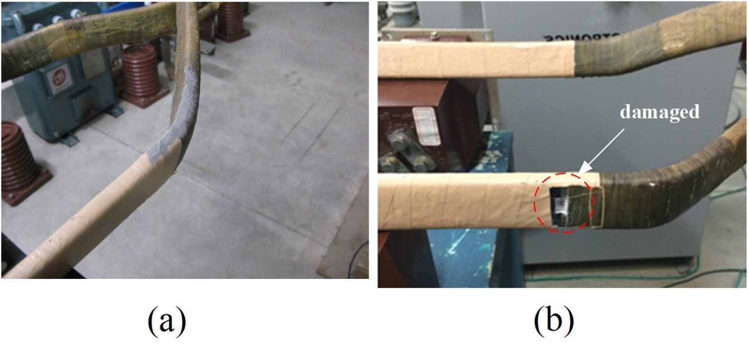
According to the International Electrotechnical Commission (IEC) standard,⁸ the electric discharge on the surface is caused by the contamination of the end winding caused by dust or conductive particles. Therefore, we follow the research studies in the literature to develop the experimental model: the conducting medium is sprinkled onto the experimentation model to simulate the electric discharge path on the bar. The effect on the defect simulation is shown on Figure 1(a).

Figure 1.

The insulation between the slot part and the end that is damaged.

Discharge in the intersecting faces of insulation

This type of defect belongs to the junction between the insulation of the slot windings and the insulation of the end windings. When the insulation damage occurs, it causes the electric discharge phenomenon.⁹ The simulation of defect is as shown in Figure 1(b).

Internal discharge of insulation

The types of internal defects can be divided into two types: internal hole and internal stratification. When we measure the bar, we found that its characteristic signal has the internal electric discharge phenomenon.¹⁰ During the thermoplastic process in manufacturing the bar, a small amount of porosity inside the bar may be produced that causes the discharge phenomenon.

Outline of artificial neural network

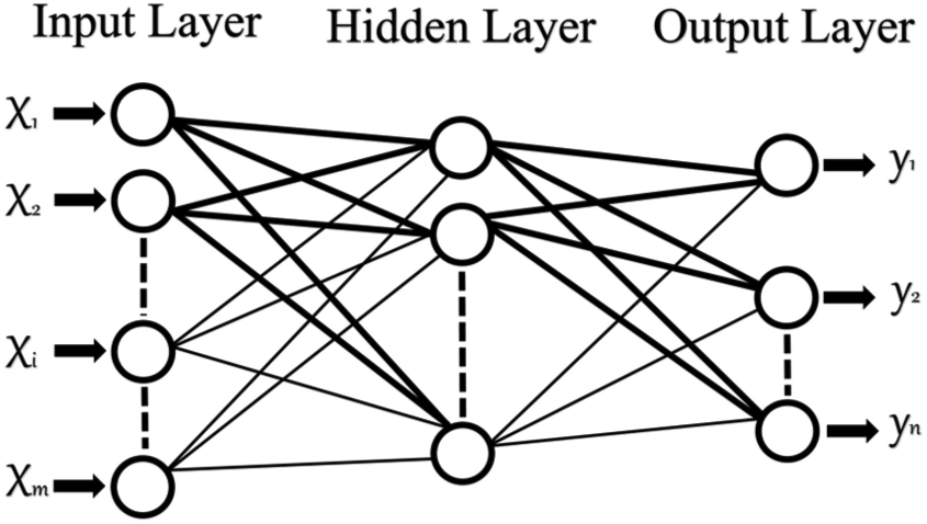
The most basic unit of the artificial neural network is an artificial neuron, also called the process element (PE) or node. The path of transmission of the signal between the processing units is called a connection. Every connection has a weight W_ij, which represents the influence of the ith neuron to the jth neuron. The artificial neural network is composed of many artificial neurons (PE) that are connected to each other.¹¹ The most common network topology uses the forward network, which contains many layers, as shown in Figure 2. The network is composed of three different layers (wherein each layer contains a number of processing units): the input layer, the hidden layer, and the output layer. Each processing unit operates in parallel independently. The input neurons are used to receive the outside signals and inject the signal into the neural network. The hidden neurons, often containing several layers, are used to process the signals from the input layer. The neurons of the output layer are used to accept the processed signals from the network and send the signals outside.¹²

Figure 2.

Truss of the back-propagation network.

In the project, we use one hidden layer for this application. In this study, we performed experiments using one hidden layer, two hidden layers, and three hidden layers. These experiments showed that these three cases yielded nearly identical results. Considering the computational ability of computers and the degree of calculating complexity, we decided to use one hidden layer for this application.

Process of analysis of partial discharge

Measurement of the signal

The signal of the partial discharge that we are considering often occurs in the high-frequency band.¹³ Thus, we set the sampling frequency of the high-frequency current sensor to 20 MS/s to measure the partial discharge signal. Next, we take a 60-Hz power supply and compare its signal to obtain the phase angle. Three cycles, which are approximately 0.05 s in total, are used to measure the original pulse signal. The three complete cycles have 1 million data points.

Hilbert–Huang transform

Empirical mode decomposition

The analysis process of the Hilbert–Huang transform does not pre-set any of the base functions. Instead, the use of the signal screening method known as empirical mode decomposition breaks down the signal into several components by a built-in modal function that is suitable for analysis of non-stationarity signal. We can use this method to show the original physical characteristics of the signal. The instantaneous frequency is an indispensable factor in the built-in modal function. The necessary condition for the instantaneous frequency is that the function is symmetric with respect to the local zero mean value. The extrema are consistent with the number of zero-crossings. Dr E. Huang and other researchers proposed the empirical mode decomposition method. The basic concept is to dismantle the signal into a number of built-in modal function components. These signals must meet the following conditions:¹⁴

The signal must have at least two extremes: one maximum and one minimum.

The signal of the characteristic time scale is defined as the difference between the times of the two extremes.

If the signal has a reverse point but does not have an extreme point, then the signal must be differentiated once or more times to obtain the extreme value, and then the component can be obtained by integrating the result.

If the signal satisfies the above the conditions, then the signal can be decomposed into built-in modal function components by empirical mode decomposition. Assuming the original signal is X(t), the process of empirical mode decomposition is shown in Figure 3.

Figure 3.

Truss of the back-propagation network.

Hilbert–Huang transform

David Hilbert was the German mathematician who proposed the Hilbert transform. He highlighted that, in the signal analysis process, the signal must start from zero time domain; otherwise, if the calculated instantaneous frequency is a negative value, it will not have a physical meaning. To solve this problem, Dr Huang proposed the method of empirical mode decomposition. The purpose of the establishment of the built-in modal function is to improve the Hilbert transform according to the constraints of the instantaneous frequency. The Hilbert–Huang transform uses the Hilbert transform to find the components of the built-in modal function and calculate the instantaneous frequency and amplitude. The Hilbert transform is defined as any time series X(t), where X(t) can be the original signal or any component of the built-in modal function. The Hilbert transform Y(t) is given by¹⁵

Y (t) = \frac{1}{π} P \int \frac{X (t')}{t - t'} dt'

(1)

where P and Z(t) are the Cauchy principal value and the Parsed signal, respectively. Z(t) is a conjugate complex number combination of X(t) and Y(t)

Z (t) = X (t) + Y (t) = a (t) e^{i θ (t)}

(2)

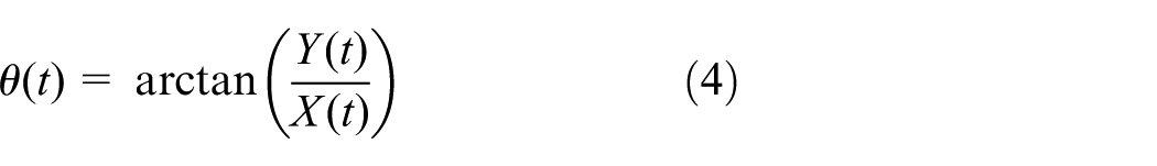
Thus, the instantaneous amplitude and instantaneous phase angle are as follows

a (t) = {[X^{2} (t) + Y^{2} (t)]}^{\frac{1}{2}}

(3)

θ (t) = \arctan (\frac{Y (t)}{X (t)})

(4)

After the instantaneous phase angle is differentiated to obtain the instantaneous frequency, the following is obtained

ω (t) = \frac{d θ (t)}{dt}

(5)

Equation (5) can be reduced to

X (t) = Re \sum_{j = 1}^{n} a_{j} (t) e^{i \int ω_{j} (t) dt}

(6)

In equation (6), a_j is the amplitude of the jth intrinsic mode function (IMF) at time t, and Re is the real component of the signal. Equation (6) can indicate that the amplitude and the frequency function of the signals change over time. The data via Fourier expansion are

X (t) = \sum_{j = 1}^{\infty} a_{j} e^{i ω_{j} t}

(7)

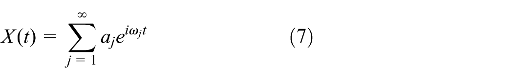
In the equation above, a_j and ω_j are constants. Comparing equations (6) and (7), we find that the IMF is a generalized Fourier expansion; the amplitude and frequency of the signal change can be clearly separated. The non-stationarity signal analysis is used to improve the Fourier transform, which can only be used for constant frequency and amplitude. In addition, equation (6) shows that the amplitude and frequency of the signal change over time and represents a three-dimensional (3D) Hilbert spectrum (H (ω, t)), also known as the Hilbert energy spectrum. According to the time integration by the Hilbert spectrum, we can obtain the relationship between the amplitude and the frequency; this relationship is called the marginal spectrum (h (ω)), given by

h (ω) = \int_{0}^{T} H (ω, t) dt

(8)

In the above equation, T is the total length of the signal, and h (ω) describes the amplitude distribution of each frequency in the entire signal. The wavelet transform is also commonly used in the time–frequency analysis. We obtain the time–frequency pattern by using the wavelet transform and the Hilbert transform and compare which is superior among the two. A clear frequency and amplitude change can be obtained from the Hilbert energy spectrum under the same resolution. We use this pattern as a follow-up analysis in the experiment.

Fractal theory—feature extraction

Fractal dimension

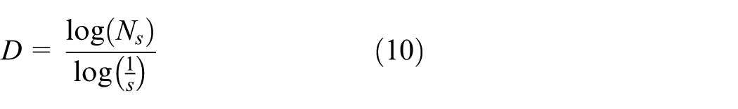
Mathematician B. B. Chaudhuri proposed the image dimension estimation method based on differential box-counting (DBC); his research proved that the algorithm has high-efficiency characteristics. The DBC is based on self-similarity. Assume that a unit fractal set is A, which consists of N_s detail self-similarity,¹⁶ and the scaling ratio is s; their relative relationship can be expressed as

N_{s} s^{D} = 1

(9)

where D is the fractal dimension and can be expressed as

D = \frac{\log (N_{s})}{\log (\frac{1}{s})}

(10)

According to definition of fractal dimension, we consider a 3D x, y, z space, where x and y are the surface positions, and z indicates the image intensity. Based on the grid computing approximate dimension, we divide a 3D space into various sizes of $L \times L \times L'$ boxes, where L is the length of measurement, and calculate the number of boxes that the image intensity surface contains. Assuming that the planned image plane is a matrix of M × M, the image plane is divided into L × L meshes according to the method described above, where the limit for L is $(M / 2) \geq L > 1$ . The size of each grid stack is an $L \times L \times L'$ box. If the minimum gray scale is in the kth box and the maximum gray scale is in the first box, then the number of boxes required for the change in gray scale change in the grid is calculated by using equation (11), and the number of boxes required for the entire image intensity surface is given by equation (12)

n_{s} (i, j) = l - k + 1

(11)

N_{s} = \sum_{i, j} n_{s} (i, j)

(12)

The number of boxes covered by the gray scale intensity surface is calculated. If the maximum gray scale in the grid is found in the fourth box and the smallest gray scale is found in the second box, then the number of boxes is estimated as

Ns = 4 - 2 + 1 = 3

Finally, by least squares method, x and y is $[\log (1 / s), \log (N_{s})]$ . The fractal dimension of the image intensity surface is the slope of the straight line, $s = L / M$ .

Lacunarity

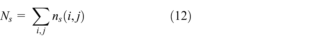
The fractal dimension of the image can be clearly calculated by the abovementioned DBC method. However, if there are two distinct fractal geometries, then they may have the same fractal dimension. Therefore, in this article, the lacunarity is considered as the auxiliary characteristic of geometric objects. Lacunarity can represent the degree of denseness of an image surface distribution as a number. When the partial discharge pattern is used for lacunarity analysis, the patterns must be normalized into binary images. If there is an M × M binary image in the pattern, where the binary image is sampled by the range covered by moving L × L boxes, then the frequency of each moving box containing m points is calculated as Q(m, L). The frequency distribution expressed as a probability equation¹⁷

P (m, L) = \frac{Q (m, L)}{N (L)}

(13)

where P(m, L) is normalized to obtain equation (14), and N is the number of points in the box

\sum_{m = 1}^{N} P (m, L) = 1

(14)

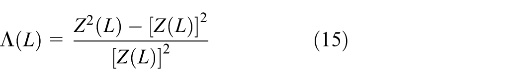
The first-order momentum Z(L) and the second-order momentum Z²(L) are calculated from the statistical moments of the probability distribution, and the lacunarity is calculated from the first-order momentum and the second-order momentum, as shown below

Λ (L) = \frac{Z^{2} (L) - {[Z (L)]}^{2}}{{[Z (L)]}^{2}}

(15)

and

{\begin{matrix} Z (L) = \sum_{m = 1}^{N} mP (m, L) \\ Z^{2} (L) = \sum_{m = 1}^{N} m^{2} P (m, L) \end{matrix}

(16)

The result of the fractal feature extraction method

This study measures 30 data points for each defective test model; thus, five test models result in the measurement of 150 data points. The distribution of fractal dimension and lacunarity is extracted from the Hilbert energy pattern by using the abovementioned fractal feature extraction method shown in Figure 4. The situation of the internal insulated defects is special; such defects can be divided into two categories: internal insulation holes and internal insulation stratification. From the patterns found from the internal insulation holes and the internal insulation stratification, the distribution characteristics of the patterns are found to be similar. The difference between the two is that the signal discharge of the insulated internal stratification is higher than the signal discharge of the insulated internal hole. After the fractal feature is extracted, the feature distribution became closer. Therefore, these two types of insulation defects are classified as the same in this experiment. The following are the insulation bar status classification types.

Type 1: The status of the normal bar insulation.

Type 2: Electric discharge of the slot.

Type 3: Electric discharge from the end winding surface.

Type 4: Electric discharge at the junction of the end insulation.

Type 5: Internal insulation defects (including internal holes and internal stratification).

Figure 4.

Types of the test of the distribution of the features of the fractal of Hilbert spectrum.

In Figure 4, the feature distribution of each defect type is different. X and Y denote the fractal dimension and the value of lacunarity, respectively. The five categories of the defective test model can be roughly separated into two fractal features, and these five types of defects form a grid. Observing the distribution of the figure, Type 1 is relatively easy to distinguish. The fractal dimension of Type 2 covers a wide range and has a longer banner area, and its fractal dimension is mostly between 1 and 2.5. Type 4 is similar to Type 2, and two types can be distinguished by lacunarity. Type 3 and Type 5 are observed by fractal feature extraction, and both of the patterns are similar in discharge area. Therefore, after the pattern data are solved by the fractal theory, it is possible to extract a small number of key features from the complex Hilbert energy pattern. Five types of discharge clustering are produced depending on the defect types of different discharge characteristics.

Artificial neural network–pattern recognition

Conjugate gradient algorithm

The basic back-propagation algorithm concept is to adjust the weight value in the steepest descent direction (also known as the negative gradient direction). The method achieves the fastest decline in the performance function but may not necessarily produce the fastest convergence. However, the conjugate gradient algorithm is used to find the size of steps along the conjugate direction to ensure the performance function can be minimized along this direction.

The conjugate gradient algorithm begins on the first iteration by searching the steepest descent, as follows

p_{0} = - g_{0}

(17)

g_{k} \equiv {\nabla F (x) |}_{x = x_{k}}

(18)

where x_k is the parameter vector (including the weight value and bias) at the kth iteration. Next, the line search determines the nearest distance along the negative gradient direction as follows

x_{k + 1} = x_{k} + α_{k} p_{k}

(19)

The next search direction must be the conjugate of the previous direction. Determining the new search direction involves the following general steps. The previous search direction and the new steepest decline direction are combined as follows

p_{k} = - g_{k} + β_{k} p_{k - 1}

(20)

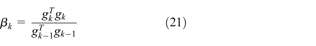
Next, the parameter β_k of the conjugate gradient algorithm must be updated; it can be obtained by

β_{k} = \frac{g_{k}^{T} g_{k}}{g_{k - 1}^{T} g_{k - 1}}

(21)

However, the conjugate gradient algorithm requires a line search in each iteration, causing the calculation time to be large. A line search requires the network to search for each line to calculate all the training input times; this process consumes a lot of time. Moller developed a new scaled conjugate gradient (SCG) algorithm that can improve time-consuming line searches. The model-trust region method and conjugate gradient method are combined to create a new algorithm that can improve the search speed of the conjugate gradient method.

Quasi-Newton algorithm

Newton’s algorithm is faster than the conjugate gradient method and is another option for rapid optimization. The basic steps of the algorithm are as follows

x_{k + 1} = x_{k} - A_{k}^{- 1} q_{k}

(22)

A_k represents the Hessian matrix, which is the second derivative of the current weight value and the bias for the performance target

A_{k} \equiv {\nabla^{2} F (x) |}_{x = x_{k}} and g_{k} \equiv {\nabla F (x) |}_{x = x_{k}}

(23)

The convergence rate of this method is faster than the conjugate gradient method. Because the Hessian matrix computational network requires much time, the quasi-Newtonian algorithm was derived. The Newton algorithm does not need to calculate the quadratic differential and update the approximate objective function with each iteration. The repeated action is a gradient function.

Levenberg–Marquardt algorithm

The main idea of the Levenberg–Marquardt method (LM method) is to combine the advantages of the Newton algorithm with the advantages of back-propagation network. The search direction of the initial iteration is prone to move toward the direction of the gradient; this approach is called the steepest descent method. The Newton method provides the direction according to the parameter μ to control the convergence speed when the iteration is in the middle and later. If μ is large, then the LM method will have the steepest slope (gradient steepest descent) characteristics. If μ is very small, then it will have the characteristics of the Newton method. When the two advantages are combined, the new weight formula obtained by the LM method is as follows

x_{k + 1} = x_{k} - {[J^{T} J + μ I]}^{- 1} J^{T} e

(24)

where J is the Jacobian matrix, which contains the network error for the first-order differential of the weight value and bias; I is the element matrix; and e is the network error vector.

Experimental results and discussion

Summary of the artificial neural network

In this article, the architecture of the artificial neural network is a three-layer feed-forward back-propagation transfer network. The transfer function in the hidden layer adopts a hyperbolic tangent function. The transfer function in the output layer uses a double-bending function. The number of neurons in the output layer is five, representing five partial discharge defect models. Types 1–5 represent the five discharge models. The values representing these five discharge models are (1,0,0,0,0), (0,1,0,0,0), (0,0,1,0,0), (0,0,0,1,0), and (0,0,0,0,1). The total number of training samples is 30, and total number of identifying samples is 10. The output value is shown in Table 1.

Table 1.

Description of the experimental model and the target output.

Model number	Test data		Target output
	Training	Identification
Type 1	Normal	30	10	1	0	0	0	0
Type 2	Slot discharge	30	10	0	1	0	0	0
Type 3	Creeping discharge	30	10	0	0	1	0	0
Type 4	Interface discharge	30	10	0	0	0	1	0
Type 5	Internal discharge	30	10	0	0	0	0	1

Discussion of the different algorithms for the artificial neural network

There are different recognition effects when using different algorithms on the artificial neural network. There are three common learning methods for test comparison that aim at a common algorithm of artificial neural network: SCG, Broyden-Fletcher-Goldfarb-Shanno (BFGS) Quasi-Newton and LM. Here, we discuss the influences of different calculation methods for defect identification. The number of neurons in the input layer of the artificial neural network is fixed at 30. The number of neurons in the output layer is five, expressed as the five partial discharge models: Type 1, Type 2, Type 3, Type 4, and Type 5. The hidden layer uses 10 neurons. Each training process is finished when the number of learning cycles reaches 10,000. There are 10 verification data points, and each data point is checked 10 times. There are total of 100 data points under the same structure. The identification results for the different number of hidden neurons are shown in Table 2.

Table 2.

The identification results of algorithm for different discharge models.

		The number of neurons in the hidden layer
		SCG	BFGS	LM
Test model	Type 1, (%)	90	79	85
	Type 2, (%)	80	69	79
	Type 3, (%)	84	79	82
	Type 4, (%)	87	72	87
	Type5, (%)	94	81	82
Total recognition rate, (%)		87	76	83
Average operation time, (s)		43	50	47
Maximum operation time, (s)		84	92	98

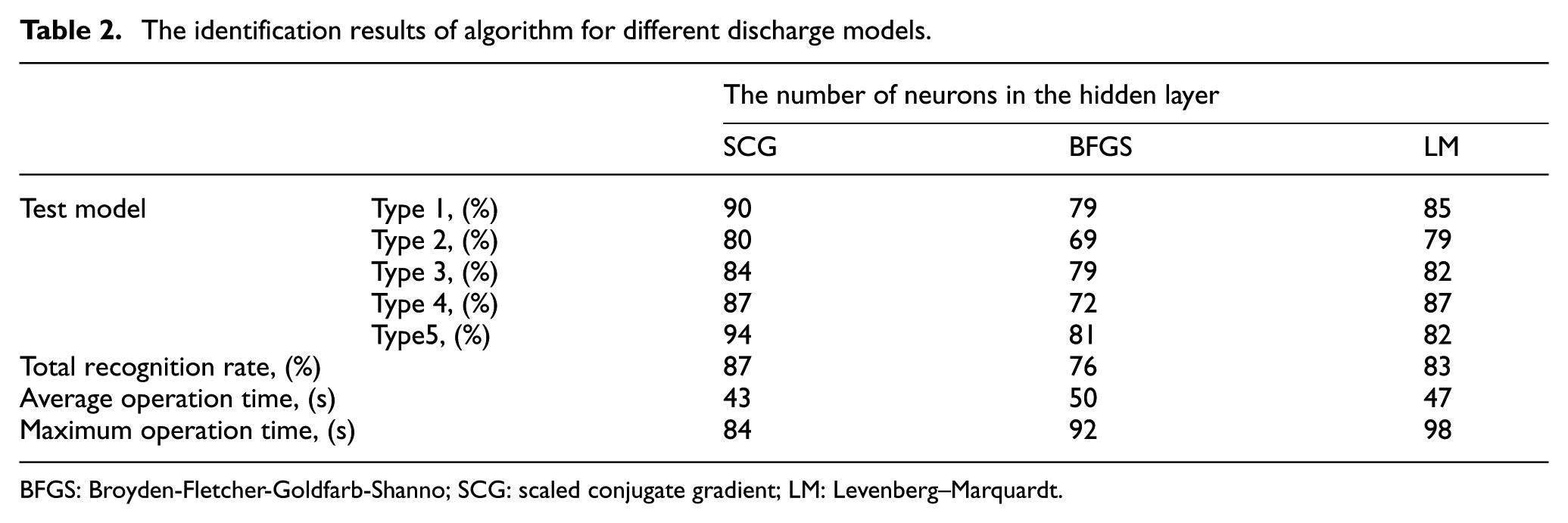
BFGS: Broyden-Fletcher-Goldfarb-Shanno; SCG: scaled conjugate gradient; LM: Levenberg–Marquardt.

It can be found from Table 3 that the neuron uses different algorithms and that there are different identification results. It can be seen from the table that the conjugate gradient algorithm has the best recognition effect, which is 87%, followed by 83% of the LM algorithm, and 76% of the pseudo-Newton algorithm. The conjugate gradient algorithm has the best recognition result.

Table 3.

The identification discharge model results of different number of neurons in the hidden layer.

		The number of neurons in the hidden layer
		5	10	20	30	40
Test model	Type 1, (%)	78	90	90	86	81
	Type 2, (%)	74	80	87	75	72
	Type 3, (%)	77	84	91	84	79
	Type 4, (%)	81	87	91	87	80
	Type5, (%)	81	94	93	82	83
Total recognition rate, (%)		78	86	91	82	79
Average operation time, (s)		31	43	48	64	76
Maximum operation time, (s)		71	84	104	112

Another focus of the discussion is the operation time speed. This is one of the criteria used to identify whether the system is good or poor. Because the speed of the SCG method is the fastest method and the longest operation time of SCG is shorter than those of the other learning methods, the SCG method is the most suitable for the problem calculation method.

Conclusion

In this study, we used four different insulation stator bars with defects and a normal insulation stator bar to establish five types of models. The five types of original signals were processed by Hilbert–Huang pattern transform. The intensity of the discharge and the distribution were observed, and the energy pattern was accessed. The feature extraction method was used to extract the important features of the pattern. The features were used for the input layer data of the artificial neural network structure to establish the defect type database of the partial discharge of the high-voltage motor. In this study, the back-propagation network architecture used three learning methods to simulate the pattern recognition system. It is concluded that the recognition rate of the conjugate gradient algorithm is higher than that of LM method and quasi-Newton method. The conjugate gradient method was used to analyze the increasing number of neurons in the hidden layer for the identification system to determine whether there is a better recognition rate and operation speed. The results indicated that, when the number of neurons is 20, the total recognition rate is 90% and is the highest. If we can collect more complete discharge defect pattern data in the future, then the study of the pattern identification system will have accurate results.

Footnotes

Handling Editor: Stephen D Prior

Declaration of conflicting interests

The author(s) declared no potential conflicts of interest with respect to the research, authorship, and/or publication of this article.

Funding

The author(s) disclosed receipt of the following financial support for the research, authorship, and/or publication of this article: This document is supported by the Ministry of Science and Technology for supporting research funding (program numbers: MOST 105-2221-E-011-081-MY3 and MOST 105-2221-E-011-082-MY3). The authors hereby express their thanks for their support.

ORCID iD

Cheng-Chien Kuo

References

High-voltage test techniques Partial discharge measurements: CNS 15175, 2008, http://tavanayrianik.ir/IEC.60270.2000.BRITISH.pdf

Wang

Hang

. Motor failure diagnosis based on ant colony algorithm and BP neural network. Noise Vib Worldw 2011; 42: 51–56.

Stone

Goodeve

. Unusual PD pulse phase distributions in operating rotating machines. IEEE T Dielect El In 1995; 2: 567–577.

Nikranjbar

Ebrahimi

Wood

. Model-based fault diagnosis of induction motor eccentricity using particle swarm optimization. Science 2008; 223: 607–615.

Lévesque

David

Hudon

. Effect of surface degradation on slot partial discharge activity. IEEE T Dielect El In 2010; 17: 1428–1440.

Hudon

Bélec

Lévesque

. Study of partial discharges in air-cooled generators. IEEE T Dielect El In 2008; 15: 1675–1690.

. Defects identification on the stator winding insulation of high-voltage motor using partial discharge measurement. MSc Thesis, Department of Electrical Engineering, National Taiwan University of Science and Technology, Taipei, Taiwan, 2015.

IEC TS 60034-27:2006. Rotating electrical machines—Part 27: Off-line partial discharge measurements on the stator winding insulation of rotating electrical machines.

Nguyen

Lee

. Improvement of induction motor fault diagnosis performance by using genetic algorithm-based feature selection. Science 2008; 222: 1613–1619.

10.

Bradley

Mason

Pezouvanis

et al . A sensorless speed estimation algorithm for use in induction motor fault detection applications. Proc IMechE, Part I: J Systems and Control Engineering 2013; 228: 257–264.

11.

Zhao

Yang

et al . Modularized fault diagnosis model of induction motor based on radial basis function neural network. Engineering 2014; 229: 3–10.

12.

Hagan

Demuth

Beale

. Neural network design, 1996. PWS Pub.

13.

Niu

Son

Yang

AWB

et al . A comparison of classifier performance for fault diagnosis of induction motor using multi-type signals. Struct Health Monit 2007; 6: 215–229.

14.

Huang

Shen

Long

et al . The empirical mode decomposition and the Hilbert spectrum for nonlinear and non-stationary time series analysis. P Roy Soc A: Math Phy 1998; 454: 903–995.

15.

Huang

Shen

Long

. A new review of nonlinear water waves: the Hilbert spectrum. Annu Rev Fluid Mech 1999; 31: 417–457.

16.

Mandelbrot

. The fractal geometry of nature. New York: W.H. Freeman publishers, 1983.

17.

Satish

Zaengl

. Can fractal features be used for recognizing 3-d partial discharge patterns. IEEE T Dielect El In 1995; 2: 352–359.

Partial discharge detection for stator winding insulation of motors using artificial neural network

Abstract

Keywords

Introduction

Introduction of the background of partial discharge and the artificial neural network

Insulation defect model of the stator coil in thehigh-voltage motor

Internal discharge of insulation

Internal hole

Internal stratification

Insulated discharge of the external part

Surface discharge

Discharge in the intersecting faces of the insulation

Slot of electric discharge

Introduction of the test model

Coil insulation of the normal stator

Slot of electric discharge

Electric discharge of end winding of insulation

Insulated discharge of the external parts

Discharge in the intersecting faces of insulation

Internal discharge of insulation

Outline of artificial neural network

Process of analysis of partial discharge

Measurement of the signal

Hilbert–Huang transform

Empirical mode decomposition

Hilbert–Huang transform

Fractal theory—feature extraction

Fractal dimension

Lacunarity

The result of the fractal feature extraction method

Artificial neural network–pattern recognition

Conjugate gradient algorithm

Quasi-Newton algorithm

Levenberg–Marquardt algorithm

Experimental results and discussion

Summary of the artificial neural network

Discussion of the different algorithms for the artificial neural network

Conclusion

Footnotes

Declaration of conflicting interests

Funding

ORCID iD

References