Sage Journals: Discover world-class research

Abstract

The performance of a vehicle in minimum time handling is highly important for the safety of the vehicle. In this study, a vehicle motion state equation with 3 degrees of freedom was established on the basis of the lateral, yaw, and longitudinal motions of the vehicle. Equations on the linear tire and motion trajectory were established with consideration of longitudinal load transfer to establish the vehicle-handling dynamics model. Steering-wheel angle, driving force equation set, and yaw angle equation had been introduced to convert the vehicle-handling dynamics model into the vehicle-handling inverse dynamics model. By introducing performance index, control set, and several constraint conditions, an optimal control model of the vehicle minimum time handling was established, which was solved by improved direct multiple-shooting nonlinear programming method. A comparison of the simulation results of ADAMS/Car and MATLAB showed that both of the optimal routes input were in tangent with the road boundary. We can observe through the longitudinal velocity that the MATLAB simulation results are more similar to a straight line than that of the ADAMS/Car simulation results, which meet the psychological expectation of a driver. Thus, the inverse dynamics model on minimum time handling of the vehicle is reasonable and feasible.

Keywords

Vehicle minimum time handling inverse dynamics sequential quadratic programming optimal control

Introduction

Vehicle-handling stability under high speed determines the safety and driving performance of a vehicle. The safety of vehicle is a social focus issue. Thus, vehicle-handling stability under high speed is a significant research topic. Currently, two methods are used in the research on vehicle-handling stability: one is called open loop and the other is called closed loop. In the open-loop method, feedback from the driver is not considered, whereas in the closed-loop method, the driver model parameter is difficult to identify. In order to solve the bottleneck problem in the modeling of the driver, corresponding research has been conducted on vehicle-handling inverse dynamics since the mid-1980s.

In vehicle-handling inverse dynamics, which belongs to the inverse problem in dynamics, the vehicle under high-speed driving is taken as a research object. The aim is to obtain the permissible driver-handling input based on the already known vehicle-handling dynamics model and vehicle motion response. The method of vehicle-handling inverse dynamics, which calculates the handling input for the driver under the designated handling performance, is different from vehicle-handling dynamics. The designated handling performance refers to passing through the given route at the fastest possible speed and not deviating from the given route boundary, thereby taking the shortest time; this issue reflects the minimum time-handling problem.

Fujioka and Kimura¹ used the simple vehicle transient dynamics model to express vehicles with different driving means and different steering configurations. They used the conjugate gradient descent to solve the problem of minimum time handling whose start point, end point, and trace were not constrained. However, this problem was not universal. Using the optimal control theory and Pontryagin’s minimum principle, Hendrikx et al.² investigated the problem of minimum time and optimal handling based on vehicle dynamic model with 2 degrees of freedom (DOFs). An adjoint equation should be established by using this method and then transformed to a nonlinear two-point boundary value problem. The major limitation was that although robustness could be achieved for the imprecise start point by using gradient descent to solve the optimal control problem, the convergence rate was slow. Casanova et al.^3–5 studied the problem of minimum time handling. Although the general solution was not provided, sequential quadratic programming algorithm was tried to solve the constrained minimum value of a multivariable function. With regard to the effect of yawing moment of inertia on vehicle performance under double-lane handling, the conclusion is that the yawing moment of inertia has little impact on vehicle minimum time handling. This conclusion was significant to vehicle design. Timings et al.^6–8 used convex programming to establish a time-varying aiming controller based on the nonlinear vehicle model; the steering-wheel handling of driver was optimized under a constant forward vehicle speed, thereby enabling the vehicle to pass the route within the shortest time, and also establishing the driver controller. However, only 2 DOFs on lateral and yawing and nonlinear tire were considered in establishing the vehicle model, and arithmetic of solving the convex programming problem was relatively complicated. Zhang and colleagues^9,10 preliminarily researched driver-handling input identification and optimal velocity curve line in the problem of minimum time handling by using 2 DOFs vehicle dynamics model based on optimal control theory. But the proposed model is imperfect. Bunte et al.¹¹ studied the optimal sideslip angle in tracking the designated yaw rate. Velenis and Colleagues^12–14 studied the optimal velocity curve by semi-analytical method in the case of maximum acceleration limit. Limebeer et al.¹⁵ solved the optimal control problem of a Formula One car using the orthogonal collocation method. This method can optimize the use of the driver controller, such as steering, braking, and accelerating, and can optimize the parameters of the vehicle. Liu and colleagues^16,17 proposed a new technique for vehicle-handling inverse dynamics; this technique is called Gauss pseudo-spectral method, which can objectively evaluate performance in emergency collision avoidance. Qiu¹⁸ conducted a simulation study on handling inverse dynamics on the conditions of high-speed vehicle emergency avoidance using radial basis function neural network and the optimal control method, with a 3-DOF vehicle-steering model as the object.

The aforementioned researches studied the path tracking, optimal velocity, and optimal sideslip angle problems. Results have shown that using the vehicle-handling inverse dynamics method to study vehicle-handling performance is feasible. Only a few experts^1–10 have studied the minimum time-handling problem, but their research hypotheses were far from the actual conditions, and the research model was imperfect. Thus, the research results were difficult to apply in practice.

In this study, under the vehicle-handling dynamics model, the front-wheel angle, driving force equation, and yaw equation have been introduced, and the vehicle-handling dynamics model has been transformed into the vehicle-handling inverse dynamics model. By introducing performance index, control set and several constraint conditions, we can establish the optimum control model of vehicle minimum time handling. By comparing the simulation results of ADAMS/Car and MATLAB, we can verify the rationality of the vehicle minimum time-handling inverse dynamics model. Through this model, the driver steering-wheel input can be solved directly under the condition of the default driver model, thus skillfully avoiding all kinds of problems of driver model in the vehicle-handling dynamics. The driver steering-wheel input obtained can provide guidance to the driver overtaking process how to manipulate the steering wheel, can provide technical support for driverless vehicles research and can provide guidance for racing training. The research has opened up a new idea for automotive engineers and provided a theoretical basis for optimizing the design of vehicles and intelligent vehicles research.

Handling dynamics model of vehicle

Equation of motion state of vehicle

Based on the assumption that the cornering properties of tires are within the linear range, the motion differential equation of the vehicle is simplified as the vehicle model that has 3 DOFs, namely, lateral motion, yawing motion, and longitudinal motion. As shown in Figure 1, the differential equation of motion state can be expressed as

{\begin{matrix} \overset{\cdot}{v} = - u ω_{r} + \frac{F_{yf} \cos δ + F_{yr} + F_{xf} \sin δ}{m} \\ {\overset{\cdot}{ω}}_{r} = \frac{a F_{yf} \cos δ - b F_{yr} + a F_{xf} \sin δ}{I_{z}} \\ \overset{\cdot}{u} = v ω_{r} + \frac{F_{xf} \cos δ - F_{yf} \sin δ + F_{xr} - F_{f} - F_{w}}{m} \end{matrix}

(1)

where v represents the lateral velocity of the vehicle, u represents the longitudinal velocity, ω_r represents the yaw rate of the vehicle, m represents the mass of the vehicle, I_z represents the moment of inertia of the vehicle surrounding the vertical axle, a represents the front wheelbase, b represents the rear wheelbase, δ represents the front-wheel angle, F_yf represents front-wheel cornering force, F_yr represents rear-wheel cornering force, F_xf represents front-wheel driving force/brake force (F_xf ≥ 0 represents driving force and F_xf < 0 represents brake force), F_xr represents rear-wheel driving force/brake force, F_f represents rolling resistance (F_f = fmg, where f represents rolling resistance coefficient), F_w represents air resistance (F_w = C_DA(3.6u)²/21.15, C_D represents air resistance coefficient, and A represents windward area).

Figure 1.

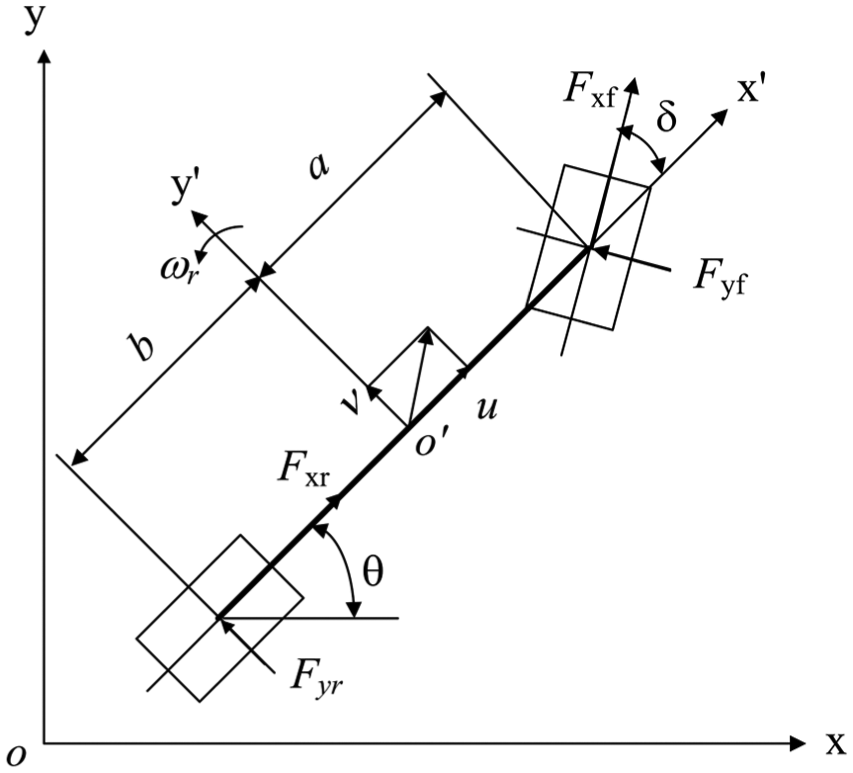
3-DOF vehicle model.

Linear tire equation

When the lateral acceleration of the vehicle is less than 0.4 g, we can assume that the tire is within linear range. The front- and rear-wheel cornering forces can be expressed as¹⁹

{\begin{matrix} F_{yf} = k_{1} (\frac{v + a ω_{r}}{u} - δ) \sqrt{1 - {(\frac{F_{xf}}{φ F_{zf}})}^{2} + {(\frac{F_{xf}}{k_{1}})}^{2}} \\ F_{yr} = k_{2} (\frac{v - b ω_{r}}{u}) \sqrt{1 - {(\frac{F_{xr}}{φ F_{zr}})}^{2} + {(\frac{F_{xr}}{k_{2}})}^{2}} \end{matrix}

(2)

where k₁ represents the cornering stiffness of the front wheel; k₂ represents the cornering stiffness of the rear wheel; φ represents friction coefficient on road surface; F_zf represents front-wheel vertical force; and F_zr represents rear-wheel vertical force.

Transfer of longitudinal load

If suspension vertical vibration and roll are not considered, the following relations would exist between the loads of the front and rear wheels of the vehicle

{\begin{matrix} F_{zf} = \frac{mgb - (F_{xf} + F_{xr}) h_{g}}{a + b} \\ F_{zr} = \frac{mga + (F_{xf} + F_{xr}) h_{g}}{a + b} \end{matrix}

(3)

where h_g represents the height of the vehicle mass center.

Equation of motion trace

To calculate the motion trace of the vehicle, the ground reference coordination system should be set up as oxy (Figure 1), in which the mass center coordinates of the vehicle are x and y, and the intersection angle between the vehicle coordinate x′ axle and the ground reference coordinate x axle is called yaw θ. Then, equation of the vehicle motion trace is expressed as

{\begin{matrix} \overset{\cdot}{x} = u \cos θ - v \sin θ \\ \overset{\cdot}{y} = v \cos θ + u \sin θ \end{matrix}

(4)

Handling inverse dynamics model of vehicle

By introducing the steering-wheel angle, driving force equation, and yaw angle equation, we can obtain the steering-wheel input, driving force input, and yaw of vehicle individually. Thus, the vehicle-handling dynamics model is transformed into the vehicle-handling inverse dynamics model.

Equation of front-wheel angle

The sideslip angles of the front and the rear wheels are as follows

α_{1} = \frac{v + a ω_{r}}{u} - δ, α_{2} = \frac{v - b ω_{r}}{u}

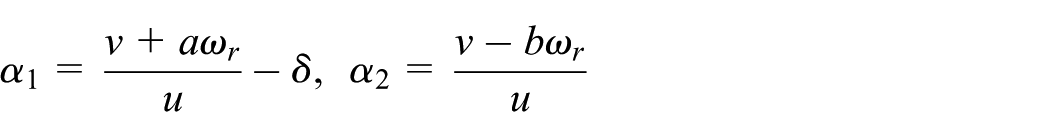
where α₁ represents front-wheel sideslip angle; and α₂ represents rear-wheel sideslip angle.

In a study by Yu,²⁰δ is expressed as $δ = L / R + (α_{1} - α_{2})$ .

where L represents the wheelbase of the vehicle, and R represents the turning radius of the vehicle.

We can obtain

δ = \frac{L}{2} (\frac{ω_{r}}{u} + \frac{1}{R})

(5)

From δ in formula (5), we can observe that the front-wheel angle is determined together by state ω_r/u and input route 1/R.

Equation set of driving force

Under minimum time handling, according to Hamilton function, the vehicle is under driving state. So F_xf > 0. A front-wheel drive vehicle has been considered in the article, and we have F_xr = 0, then putting it into formulas (2) and (3), and processing. We have

{\begin{matrix} F_{yf} = k_{1} α_{1} \sqrt{1 - {[\frac{(a + b) F_{xf}}{φ (mgb - F_{xf} h_{g})}]}^{2} + {(\frac{F_{xf}}{k_{1}})}^{2}} \\ F_{yr} = k_{2} α_{2} \end{matrix}

(6)

In the second differential equation of formula set (4), we take both sides of the derivative of $\overset{\cdot}{y} = v \cos θ + u \sin θ$ .

We have

\sum F_{y} = m \overset{\cdot\cdot}{y} = m (\overset{\cdot}{v} \cos θ - v \overset{\cdot}{θ} \sin θ + \overset{\cdot}{u} \sin θ + u \overset{\cdot}{θ} \cos θ)

(7)

According to the first differential equation of formula set (1), we have

\sum F_{y} = m \overset{\cdot\cdot}{y} = m (\overset{\cdot}{v} + u ω_{r}) = F_{yf} \cos δ + F_{yr} + F_{xf} \sin δ

(8)

Combining formulas (7) and (8), we have

\begin{array}{l} m (\dot{v} \cos θ - v \dot{θ} \sin θ + \dot{u} \sin θ + u \dot{θ} \cos θ) \\ = F_{y f} \cos δ + F_{y r} + F_{x f} \sin δ \end{array}

(9)

Putting the first and the third differential equation of formula set (1) into formula (9), we have

\begin{array}{l} F_{x f} [\sin δ - \sin (δ + θ)] + F_{y f} [\cos δ - \cos (δ + θ)] \\ + F_{y r} (1 - \cos θ) + (F_{f} + F_{w}) \sin θ = 0 \end{array}

(10)

Combining formulas (6) and (10), we have

{\begin{matrix} F_{xf} [\sin δ - \sin (δ + θ)] + F_{yf} [\cos δ - \cos (δ + θ)] + F_{yr} (1 - \cos θ) + (F_{f} + F_{w}) \sin θ = 0 \\ F_{yf} = k_{1} (\frac{v + a ω_{r}}{u} - δ) \sqrt{1 - {[\frac{(a + b) F_{xf}}{φ (mgb - F_{xf} h_{g})}]}^{2} + {(\frac{F_{xf}}{k_{1}})}^{2}} \\ F_{yr} = k_{2} (\frac{v - b ω_{r}}{u}) \end{matrix}

(11)

In formula (11), if the state variable is a known quantity, we can solve the implicit functions F_xf, F_yf, and F_yr.

Equation for yaw

The relations of yaw θ, sideslip angle of mass center β, and yaw rate ω_r are expressed as follows

θ = β + \int_{0}^{t} ω_{r} d \tilde{t}

(12)

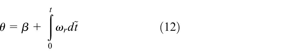
Taking the derivative of formula (12), we obtain

\overset{\cdot}{θ} = \overset{\cdot}{β} + ω_{r}

(13)

where β = v/u represents sideslip angle of mass center.

Putting the first and the third differential equation of formula set (1) into formula (13), we obtain

\overset{\cdot}{θ} = \frac{(- m v^{2} ω_{r} + (u F_{yf} - v F_{xf}) \cos δ + (u F_{xf} + v F_{yf}) \sin δ + v (F_{f} + F_{w}) + u F_{yr})}{m u^{2}}

(14)

Motion radius of vehicle

Since the item of the vehicle-steering radius exists in the steering angle equation, the vehicle radius expression should be introduced. Considering that the vehicle-steering radius is obtained from motion trace formula (4), we can obtain

\frac{dy}{dx} = \frac{v \cos θ + u \sin θ}{u \cos θ - v \sin θ}

(15)

\frac{d^{2} y}{d x^{2}} = \frac{u \overset{\cdot}{v} - \overset{\cdot}{u} v}{{\overset{\cdot}{x}}^{3}}

(16)

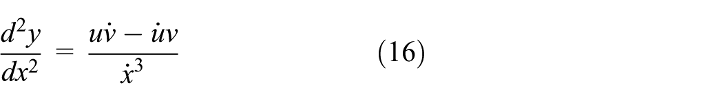
The steering radius of vehicle R can be solved as follows through knowledge of advanced mathematics

R = \frac{1}{K} = \frac{{(1 + y')}^{2}}{{y ″}^{3 / 2}}

(17)

Putting formulas (15) and (16) into formula (17), we have

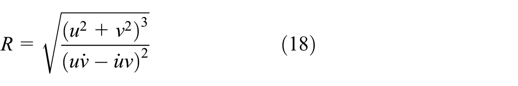
R = \sqrt{\frac{{(u^{2} + v^{2})}^{3}}{{(u \overset{\cdot}{v} - \overset{\cdot}{u} v)}^{2}}}

(18)

From the steering radius expression, we can observe that the steering radius of the vehicle is determined by motion state.

According to formula (15), we obtain

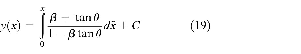
y (x) = \int_{0}^{x} \frac{β + \tan θ}{1 - β \tan θ} d \tilde{x} + C

(19)

From the initial condition y(0) = 0, we obtain C = 0. Thus

y (x) = \int_{0}^{x} \frac{β + \tan θ}{1 - β \tan θ} d \tilde{x}

(20)

Optimal control model of minimum time handling of vehicle

In the preceding sections, we have analyzed how to generate the model for vehicle dynamics. The performance index, control set, and several constraint conditions should be introduced to create the optimal control model for the minimum time handling.

Differential algebra system

For the aforementioned model, route is taken as the input and time is the value that is optimized. The displacement of vehicle should be adopted as independent variable so that the free terminal can be transformed into a fixed terminal. According to differential operation,

\frac{dy}{dt} = \frac{dx}{dt} \frac{dy}{dx} = (u \cos θ - v \sin θ) \frac{dy}{dx}

The time variable can be transformed into a displacement variable. Finally, the vehicle-handling inverse dynamics model can be sorted out as follows

\begin{array}{l} (\begin{matrix} u \cos θ - v \sin θ & 0 & 0 & 0 & 0 & 0 & 0 & 0 & 0 & 0 \\ 0 & u \cos θ - v \sin θ & 0 & 0 & 0 & 0 & 0 & 0 & 0 & 0 \\ 0 & 0 & u \cos θ - v \sin θ & 0 & 0 & 0 & 0 & 0 & 0 & 0 \\ 0 & 0 & 0 & 0 & 0 & 0 & 0 & 0 & 0 & 0 \\ 0 & 0 & 0 & 0 & 0 & 0 & 0 & 0 & 0 & 0 \\ 0 & 0 & 0 & 0 & 0 & 0 & 0 & 0 & 0 & 0 \\ 0 & 0 & 0 & 0 & 0 & 0 & 0 & 0 & 0 & 0 \\ 0 & 0 & 0 & 0 & 0 & 0 & 0 & 0 & 0 & 0 \\ 0 & 0 & 0 & 0 & 0 & 0 & 0 & 0 & 1 & 0 \\ 0 & 0 & 0 & 0 & 0 & 0 & 0 & 0 & 0 & u \cos θ - v \sin θ \end{matrix}) (\begin{array}{l} v_{x} \\ ω_{x r} \\ u_{x} \\ \frac{d F_{x f}}{d x} \\ \frac{d F_{y f}}{d x} \\ \frac{d F_{y r}}{d x} \\ δ_{x} \\ K \\ y_{x} \\ θ_{x} \end{array}) \\ = (\begin{array}{l} f_{1} \\ f_{2} \\ f_{3} \\ f_{4} \\ F_{y f} - k_{1} α_{1} f_{5} \\ F_{y r} - k_{2} α_{2} \\ δ - L / 2 (ω_{r} / u + K) \\ K^{2} - {(u f_{1} - f_{3} v)}^{2} / {(u^{2} + v^{2})}^{3} \\ \frac{(u f_{1} - f_{3} v)}{{(u \cos θ - v \sin θ)}^{3}} \\ f_{6} \end{array}) \end{array}

(21)

where

\begin{matrix} f_{1} = \frac{F_{yf} \cos δ + F_{yr} + F_{xf} \sin δ}{m} - u ω_{r}, f_{2} = \frac{a F_{yf} \cos δ - b F_{yr} + a F_{xf} \sin δ}{I_{z}} + v ω_{r} \\ f_{3} = \frac{F_{xf} \cos δ - F_{yf} \sin δ + F_{xr} - F_{f} - F_{w}}{m} \\ f_{4} = F_{xf} [\sin δ - \sin (δ + θ)] + F_{yf} [\cos δ - \cos (δ + θ)] + F_{yr} (1 - \cos θ) + (F_{f} + F_{w}) \sin θ \\ f_{5} = \sqrt{1 - {[\frac{(a + b) F_{xf}}{φ (mgb - F_{xf} h_{g})}]}^{2} + {(\frac{F_{xf}}{k_{1}})}^{2}} \\ f_{6} = \frac{(- m v^{2} ω_{r} + (u F_{yf} - v F_{xf}) \cos δ + (u F_{xf} + v F_{yf}) \sin δ + v (F_{f} + F_{w}) + u F_{yr})}{m u^{2}} \end{matrix}

Performance index

According to optimal control theory, the control vector of minimum time handling is δ and F_xf, the performance index of minimum time handling J(Z) can be described by the following mathematical expression

J (Z) = \int_{t_{0}}^{t_{f}} dt

(22)

where t₀ represents initial time, t_f represents end time, and Z represents control vector.

Control set

For the model described in this article, we take the optimized double-lane change as control set to solve the handling input of the driver. Thus, the road model should be set up first and the acceptable route input set should be recommended to drivers. Usually, we consider using low-order smooth function to fit. The road model is presented as follows²¹

f (x) = {\begin{matrix} 0 & x \in s_{1} \\ e_{0} + e_{1} x + e_{2} x^{2} + e_{3} x^{3} & x \in s_{2} \\ B & x \in s_{3} \\ {e'}_{0} + {e'}_{1} x + {e'}_{2} x^{2} + {e'}_{3} x^{3} & x \in s_{4} \\ 0 & x \in s_{5} \end{matrix}

(23)

where B is lane change distance. The road model is shown as Figure 2.

Figure 2.

The road model.

Thus, the state variable quantity of the vehicle-handling inverse dynamics model is constrained by the boundary of double-lane change

f_{1} (x) \leq y (x) \leq f_{2} (x)

(24)

In this formula, f₁(x) and f₂(x) individually represent upper and lower double-lane change equations.

The longitudinal speed u of the vehicle-handling inverse dynamics model is limited by the maximum vehicle speed, and the front-wheel angle δ is limited by the driver’s physiological limit.

Inequality constraints

Rollover constraints

In this article, the suspension function is not considered during the modeling. Thus, the impact from the roll angle of the vehicle is neglected. The vehicle is identified by its structure parameter, and the condition for rollover only requires a threshold to be reached by lateral force and lateral acceleration. In a study by Yu,²⁰ the lateral acceleration threshold is given for vehicle not rolling over

a_{y} \leq \frac{gD}{2 h_{g}}

(25)

where D is the tread.

Constraints on front-wheel driving force

In this article, we have proved that during the minimum time handling of the vehicle, the vehicle is always on the driving state. Thus, the rear-wheel driving force F_xr = 0, and the front-wheel driving force is constrained by the ground adhesive rate.

0 \leq F_{xf} \leq \frac{φ mgb}{a + b + φ h_{g}}

(26)

The front-wheel drive F_xf is also limited by the maximum driving force provided by the powertrain. According to the relationship between engine speed and vehicle speed, the relationship between engine output torque and driving force, the relationship between the maximum driving force and the vehicle speed can be obtained by the external characteristic curve of engine.

Boundary conditions

When the vehicle is on double-lane change movement, the initial state is fixed. The terminal state is constrained by lateral displacement. Thus, the boundary condition for the model is

\begin{array}{l} v (0) = v_{0}, ω_{r} (0) = ω_{r 0}, y (0) = y_{0}, \\ θ (0) = θ_{0}, u (0) = u_{0}, y (x_{f}) = y_{f} \end{array}

(27)

Normalization of longitudinal displacement

The terminal time in the minimum time handling is uncertain, so we consider taking fixed terminal displacement as the parameter in the model. In the preceding article, we have changed the independent variable of time to displacement. To obtain the simplest form, we consider normalizing the longitudinal displacement.

We define the unitized longitudinal displacement variant as follows

\bar{x} = \frac{x - x_{0}}{x_{f} - x_{0}}

(28)

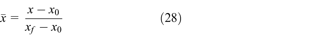
where x₀ is the initial place and x_f is the terminal place.

Taking the derivative of formula (28), we obtain

\frac{d \bar{x}}{dt} = \frac{u \cos θ - v \sin θ}{x_{f} - x_{0}}

(29)

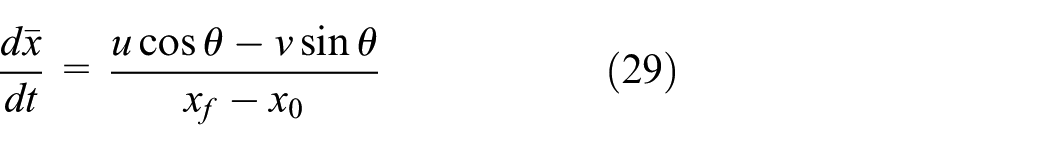
We define the new state variable

\bar{X} (\bar{x}) = {[v (\bar{x}), ω_{r} (\bar{x}), u (\bar{x}), y (\bar{x}), θ (\bar{x})]}^{T} .

Putting formula (29) into formula (22), we obtain

J (Z) = \int_{{\bar{x}}_{0}}^{{\bar{x}}_{f}} λ d \bar{x}

(30)

where $λ = (x_{f} - x_{0}) / (u \cos θ - v \sin θ)$ .

Thus, the performance index of minimum time handling is transferred to the index by taking $\bar{x}$ as variable.

The state equation (1) can be obtained in the same way, and we obtain

\frac{d \bar{X}}{d \bar{x}} = λ f [\bar{X} (\bar{x}), Z (\bar{x})]

(31)

Improved direct multiple-shooting nonlinear programming method

Transforming Lagrange problem into Mayer problem

First, we extend the dimensionality of state space, add the new variable ${\bar{X}}_{n + 1}$ and make it satisfy formula (32) through the following expression²²

{\begin{matrix} {\overset{\cdot}{\bar{X}}}_{n + 1} = λ \\ {\bar{X}}_{n + 1} (t_{0}) = 0 \end{matrix}

(32)

Thus, the performance index is transferred as

J (Z) = λ {\bar{X}}_{n + 1} (1)

(33)

Therefore, as long as we take the first formula in (32) into the system-state equation and the second formula is brought into the restraint condition, the Lagrange problem is then transformed into the Mayer problem.

Changing the Mayer problem as problem of finite-dimension nonlinear programming

Dividing the section of $\bar{x} \in [0, 1]$ as n equal parts, we obtain n + 1 node.

Setting the estimated values for control vectors at nodes, linear interpolation is conducted on the nodes and control vectors between nodes are obtained. Under an initial value of the known state variable, the equation of state is integrated, and the performance index is calculated.

Thus, the minimum time-handling inverse dynamics of the vehicle is changed as the nonlinear programming problem, which can be solved by sequential quadratic programming method.²³

Simulation results

In this article, we compare the simulation results of ADAMS/Car and MATLAB, and the rationality of the model of vehicle minimum time-handling inverse dynamics is verified. Further information on ADAMS/Car simulation is presented by Chen.²⁴

Simulation results on lateral displacement

Solving by taking fmincon function in MATLAB, Figure 3 shows the simulation results on lateral displacement along with the longitudinal displacement when the initial speed is at u = 108 km/h by using ADAMS/Car and MATLAB. The figure indicates that the optimal routes solved by the two models are consistent with each other. The characteristic of the optimal routes is that they are in tangent with the upper and lower boundaries of double-lane change and also embody the minimum principle, that is, the performance reaches its optimal value at the boundary input. A relatively larger curvature is observed in the ADAMS/Car simulation result than in the MATLAB simulation result.

Figure 3.

Simulation results on lateral displacement.

Simulation results on steering-wheel angle

Figure 4 shows the ADAMS/Car and MATLAB simulation results on the steering-wheel angle along with the longitudinal displacement. The figure indicates the goodness-of-fit of the two methods. Two peak values appeared on the steering-wheel angle in the process of overtaking. At 15 and 120 m, the steering-wheel angle is over 30°. The steering wheel nearly reaches 0° after 200 m, and then the vehicle returns to driving along the straight line.

Figure 4.

Simulation results on steering-wheel angle.

Simulation results on steering-wheel angle velocity

Figure 5 shows the ADAMS/Car and MATLAB simulation results on steering-wheel angle velocity along with the longitudinal displacement. The figure indicates that the steering-wheel angle velocity exhibits a W curve near 100 and 250 m. A relatively larger steering-wheel angle velocity appears at 20, 200, and 300 m. This angle proves that the driver is quite busy at those times.

Figure 5.

Simulation results on steering-wheel angle velocity.

Simulation results on front-wheel driving force

Figure 6 shows the ADAMS/Car and MATLAB simulation results on front-wheel driving force along with longitudinal displacement. The figure indicates that the vehicle driving force shows a convex function during the entire driving course. At the beginning, the simulation result of ADAMS/Car is larger than that of MATLAB. The MATLAB simulation result is larger than the ADAMS/Car simulation result after 50 m. During the entire overtaking process, the ADAMS/Car vehicle model has more stable driving force than the 3-DOF model established in this study.

Figure 6.

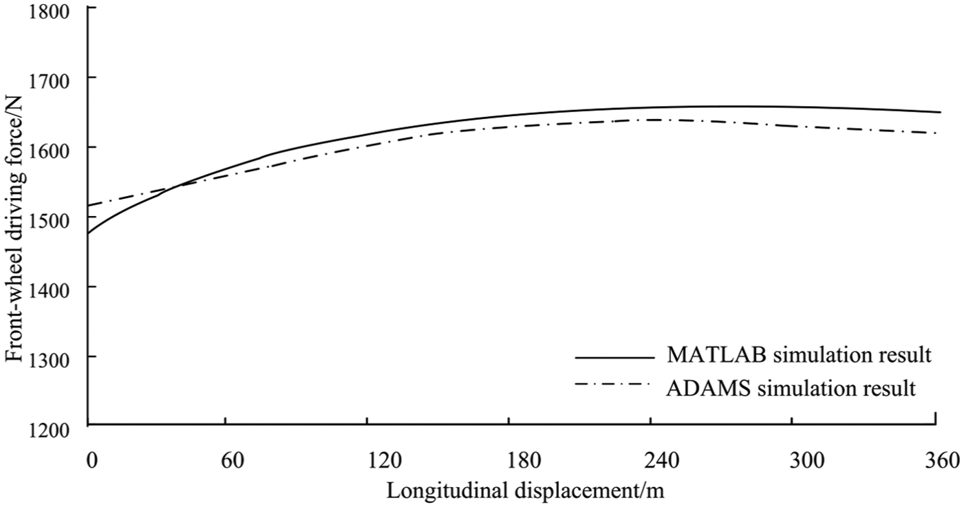
Simulation results on front-wheel driving force.

Simulation results on longitudinal velocity

Figure 7 shows the longitudinal velocity simulation results along with the longitudinal displacement by using ADAMS/Car and MATLAB. According to the figure, during the entire movement, the simulation result of MATLAB increases linearly and that from ADAMS/Car at the beginning is less than the simulation result of MATLAB. Thereafter, the ADAMS/Car simulation result is similar to the MATLAB simulation result.

Figure 7.

Simulation results on longitudinal velocity.

Conclusion

Front-wheel angle, driving force equation, yaw equation had been introduced to establish the vehicle-handling inverse dynamics model. By introducing performance index, control set, and several constraint conditions, an optimal control model of the vehicle minimum time handling was established. By comparing the virtual prototype simulation tests of ADAMS/Car and the simulation results of MATLAB, this study shows that the optimal routes from the two tests are all in tangent with the road boundary. Thus, the model meets the requirements of the minimum principle. The simulation result on the steering-wheel angle speed indicates that vibration occurs in the model, probably as a result of vibration of the linear tire. The simulation result on longitudinal speed shows that the MATLAB result resembles a straight line more than ADAMS/Car result does, and this condition meets the psychological expectation of drivers. Thus, the inverse dynamics model on minimum time handling of vehicle is reasonable and feasible.

Footnotes

Notation

a front wheelbase, m

b rear wheelbase, m

f rolling resistance coefficient

h_g height of the vehicle mass center, m

k ₁ cornering stiffness of the front- wheel, N/rad or N/(°)

k ₂ cornering stiffness of the rear-wheel, N/rad or N/(°)

m mass, kg

u longitudinal velocity, m/s

v lateral velocity, m/s

A windward area, m²

B lane change distance, m

C_D air resistance coefficient

D tread, m

F_f rolling resistance, N

F_w air resistance, N

F_xf front-wheel driving force/brake force, N

F_xr rear-wheel driving force/brake force, N

F_yf front-wheel cornering force, N

F_yr rear-wheel cornering force, N

F_zf front-wheel vertical force, N

F_zr rear-wheel vertical force, N

I_z moment of inertia of the vehicle surrounding the vertical axle, kg m²

L wheelbase, m

R turning radius, m

α ₁ front-wheel sideslip angle, rad or (°)

α ₂ rear-wheel sideslip angle, rad or (°)

δ front-wheel angle, rad or (°)

θ yaw, rad or (°)

φ friction coefficient on road surface

ω_r yaw rate, rad/s or (°)/s

Handling Editor: Mario Terzo

Declaration of conflicting interests

The author(s) declared no potential conflicts of interest with respect to the research, authorship, and/or publication of this article.

Funding

The author(s) disclosed receipt of the following financial support for the research, authorship, and/or publication of this article: This work was financially supported by the National Natural Science Foundation of China (grant no.: 51505244), the China Postdoctoral Science Foundation (grant no.: 2016M590626), the Qingdao Postdoctoral Applied Research Project (grant no.: 2015224), and the Natural Science Foundation of Shandong Province, China (grant no.: ZR2016EEM14).

ORCID iD

Li-Xia Zhang

References

Fujioka

Kimura

. Numerical simulation of minimum-time cornering behavior. JSAE Rev 1992; 13: 44–51.

Hendrikx

JPM

Meijlink

TJJ

Kriens

RFC

. Application of optimal control theory to inverse simulation of car handling. Vehicle Syst Dyn 1996; 26: 449–461.

Casanova

Sharp

Symonds

. Minimum time manoeuvring: the significance of yaw inertia. Vehicle Syst Dyn 2000; 34: 77–115.

Casanova

. On minimum time vehicle manoeuvring: the theoretical optimal lap. PhD Thesis, Cranfield University, 2000.

Casanova

Sharp

Symonds

. On minimum time optimisation of formula one cars: the influence of vehicle mass. In: Proceedings of the 5th international symposium on advanced vehicle control, Ann Arbor, MI, 22–24 August 2000, pp.585–592. London: Fisita.

Timings

Cole

. Minimum manoeuvre time of a nonlinear vehicle at constant forward speed using convex optimization. In: Proceedings of the 10th international symposium on advanced vehicle control, Loughborough, 22–26 August 2010, pp.21–26. London: Fisita.

Timings

Cole

. Efficient minimum manoeuvre time optimisation of an oversteering vehicle at constant forward speed. In: Proceedings of the 2011 American control conference, San Francisco, CA, 29 June–1 July 2011, pp.5267–5272. New York: IEEE.

Timings

Cole

. Vehicle trajectory linearisation to enable efficient optimisation of the constant speed racing line. Vehicle Syst Dyn 2012; 50: 883–901.

Zhang

Zhao

Song

. Research on inverse dynamics of vehicle minimum time maneuver problem. China Mech Eng 2007; 18: 2628–2632.

10.

Zhang

Pan

Chen

et al . Vehicle optimal velocity curves for minimum-time maneuver. Adv Mech Eng. Epub ahead of print 12 February 2014. DOI: 10.1155/2014/194868.

11.

Bunte

Sahin

Bajcinca

. Inversion of vehicle steering dynamics with modelica/dymola. In: Proceedings of the 4th international modelica conference, Hamburg, Germany, 7–8 March 2005, pp.319–328.

12.

Velenis

Tsiotras

. Optimal velocity profile generation for given acceleration limits: the half-car model case. In: IEEE international symposium on industrial electronics, Dubrovnik, 20–23 June 2005, pp.361–366. New York: IEEE.

13.

Velenis

Tsiotras

. Optimal velocity profile generation for given acceleration limits: theoretical analysis. In: Proceedings of the 2005, American control conference, Portland, OR, 8–10 June 2005, pp.1478–1483. New York: IEEE.

14.

Velenis

Tsiotras

. Minimum-time travel for a vehicle with acceleration limits: theoretical analysis and receding horizon implementation. J Optimiz Theory App 2008; 138: 275–296.

15.

Limebeer

DJN

Perantoni

Rao

. Optimal control of formula one car energy recovery systems. Int J Control 2014; 87: 2065–2080.

16.

Liu

Zhao

et al . Vehicle handling inverse dynamics based on gauss pseudospectral method while encountering emergency collision avoidance. J Mech Eng 2012; 48: 127–132.

17.

Liu

Jiang

. Optimum path-tracking control for inverse problem of vehicle handling dynamics. J Mech Sci Technol 2016; 30: 3433–3440.

18.

Qiu

. Vehicle handling inverse dynamics modeling and simulation while encountering an emergency collision avoidance. Master Thesis, Nanjing University of Aeronautics and Astronautics, 2011.

19.

Sridhar

Hatwal

. A comparative study of four wheel steering models using the inverse solution. Vehicle Syst Dyn 1992; 21: 1–18.

20.

. The theory of automobile (in Chinese). Beijing: China Machine Press, 2000.

21.

Zhang

. Research on inverse problem in vehicle handling stability and ride comfort. PhD Thesis, Nanjing University of Aeronautics and Astronautics, 2007.

22.

. Optimal control theory and method (in Chinese). Beijing: National Defense Industry Press, 2000.

23.

Yuan

Sun

. Optimization theory and methods (in Chinese). Beijing: Science Press, 1997.

24.

Chen

. Study on vehicle handling and stability evaluation based on the minimum time. Master Thesis, Qingdao Technological University, 2014.

Modeling and simulation of minimum time-handling inverse dynamics of a vehicle

Abstract

Keywords

Introduction

Handling dynamics model of vehicle

Equation of motion state of vehicle

Linear tire equation

Transfer of longitudinal load

Equation of motion trace

Handling inverse dynamics model of vehicle

Equation of front-wheel angle

Equation set of driving force

Equation for yaw

Motion radius of vehicle

Optimal control model of minimum time handling of vehicle

Differential algebra system

Performance index

Control set

Inequality constraints

Rollover constraints

Constraints on front-wheel driving force

Boundary conditions

Normalization of longitudinal displacement

Improved direct multiple-shooting nonlinear programming method

Transforming Lagrange problem into Mayer problem

Changing the Mayer problem as problem of finite-dimension nonlinear programming

Simulation results

Simulation results on lateral displacement

Simulation results on steering-wheel angle

Simulation results on steering-wheel angle velocity

Simulation results on front-wheel driving force

Simulation results on longitudinal velocity

Conclusion

Footnotes

Notation

Declaration of conflicting interests

Funding

ORCID iD

References