
Abstract
Brake system is an important actuator of most active safety systems equipped on vehicles. It combines with the wheel to make vehicle decelerate and finally stop it. Moreover, brake system is an electronic, mechanical, and hydraulic hybrid system; it contains some highly nonlinear characters, which is a challenge to system control. In this article, an integrated model of brake system and single-wheel system using bond graph method is developed, in which the nonlinear characters of the volumetric compliance effect of brake fluid and the resistance effect of valves are taken into consideration. The accuracy and reliability of the brake system is verified by experiment. Nonlinear sliding-mode controller as well as sliding-mode observer is proposed. The controller is used to modulate inlet and outlet valves control signals according to the vehicle states, which will lead to cancel the usage of wheel cylinder pressure sensors. The controller is analyzed by different tire–road friction coefficient conditions. The results show that the proposed integrated bond graph model is accurate, and the nonlinear sliding-mode control is reliable on valves control signal regulation.
Keywords
Introduction
Vehicle active safety systems have got increasing attention of the world. Active safety systems, such as anti-lock braking system (ABS), traction control system (TCS), and electronic stability control (ESC) system, enhance vehicle safety performance relied on brake system as an actuator.1–3 At present, the hydraulic brake system is widely equipped on light vehicles, in which brake fluid is used for energy transportation and conversion. Brake fluid pressure in wheel cylinder produced by driver pulls piston to press on brake disk and converts it into wheel brake torque. Wheel brake torque can make vehicle decelerate and finally stop. Moreover, these safety systems are used to improve vehicle dynamic stability on low tire–road friction coefficient road. 4
The hydraulic braking control system is an electronic, mechanical, and hydraulic hybrid system. The energy conversion and transportation of the system are realized by brake fluid. Motor pump and high-pressure accumulator are used to provide brake pressure in electro-hydraulic braking system (EHB); control valves and motor pump in hydraulic control unit (HCU) are driven by electronic energy. Most parts of the systems are mechanical components. In the hybrid system, there are some nonlinear characters, such as resistance effect of valves and the compressibility of brake fluid, which is a challenge for system control.5–7
To accurately control brake system, many control theories have been developed. Proportional–integral–derivative (PID), fuzzy control, and neural networks control are employed for brake system control and bring the system a better performance.8–10 However, these controllers are model free, 11 which would neglect some characters of system and cannot monitor states of brake system exactly. Nonlinear back stepping controller and sliding-mode controller are also developed to achieve great and robust braking performance.12,13 These control methods are nonlinear and use model-based controller.14,15 The design of model-based controller is on the basis of reference model, which would contain the characteristic of the system in controller and be more precise in system control.
Moreover, the brake system control researched mostly at present is focused on dividing the system into brake system and vehicle system and designing two controllers to control the braking system and wheel slip, respectively.16–20 CB Patil and RG Longoria 19 proposed a modularized design of an ABS and a tracking brake actuator controller, in which a sliding-mode system is used to calculate reference brake torque according to vehicle states. JJ Castillo et al. 20 developed a new fuzzy logic techniques–based controller to determine the optimum pressure in braking circuit and artificial neural network to estimate wheel slip ratio. These researches are effective, yet they would increase the usage of system states sensors, which are not applicable for integrated purpose.
In this article, an integrated model of brake system and single-wheel system based on bond graph method is proposed. The vehicle signals are used to control HCU in brake systems directly, and the wheel slip ratio is modulated. By this way, wheel cylinder pressure sensors are not necessary any more. First, an integrated model of brake system and single-wheel model based on bond graph method is established. Bond graph is a graphical method which uses energy and energy exchange to describe the dynamic systems. Using bond graph method, the systems from different domains, such as mechanical, hydraulic, and electronic, can be described in the unified way.21,22 Then, the integrated brake–wheel bond graph model is used as a reference model to design the sliding-mode controller, and the necessary system states are estimated from a sliding-mode observer. Finally, the proposed algorithm is verified by simulation.
This article is organized as follows: the first section represents the introduction of some related works. An integrated model of brake system and single wheel is established based on bond graph method in section “Integrated model,” which is used as reference model to the design of model-based controller. In section “Model validation,” a hard-in-loop system is employed to verify the correctness of brake system model. In section “Sliding-mode controller design,” sliding-mode controller is designed based on integrated bond graph model, in which the states are estimated by sliding-mode observer. Section “Simulation and analysis” presents simulation and analysis of sliding-mode controller and observer. The last section of this article is the conclusion.
Integrated model
Brake system modeling
The EHB system consists of a pedal, a master cylinder, a pedal stroke simulator, an HCU, four wheel cylinders, and some hydraulic pipes. The system contains mechanical structure, and brake fluid is used for energy conversion and transportation. Besides, the valves in HCU are driven by electronic energy. In short, it is a mechanical, electrical, and hydraulic hybrid system. Some necessary assumptions are considered for system modeling: pedal, pedal stroke simulator, master cylinder, motor pump, and high-pressure accumulator are replaced by a pressure source. Besides, the inductance, resistance, and volumetric compliance effects of brake pipe are taken into account. Bond graph method has unique advantage in hybrid system modeling. The single-circuit brake system model based on bond graph method is shown in Figure 1. It should be declared that the inlet valve is normally open and outlet valve is normally closed in conventional hydraulic braking systems, and to illustrate expediently, we assume that both of them are normally closed. The actual descriptions of elements in the bond graph are demonstrated in Table 1.23,24

Brake system model based on bond graph method.
Elements and description of brake system.

Single-wheel model
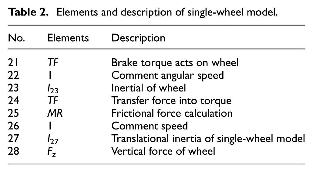
The brake torque provided by brake system acts on wheel and finally stops the vehicle, and the tire–road friction coefficient characters have significant influence on brake performance. So, another bond graph single-wheel model corresponding with single-circuit brake system is established based on the wheel structure in Figure 2. Figure 3 is the bond graph single-wheel model. The descriptions of elements are demonstrated in Table 2. 25

Single-wheel model.
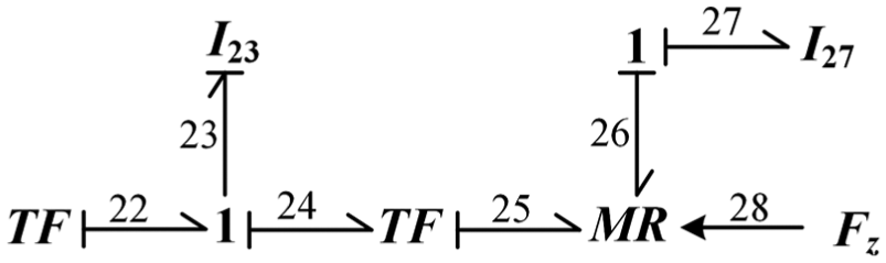
Bond graph model of single-wheel system.
Elements and description of single-wheel model.
Integrated modeling
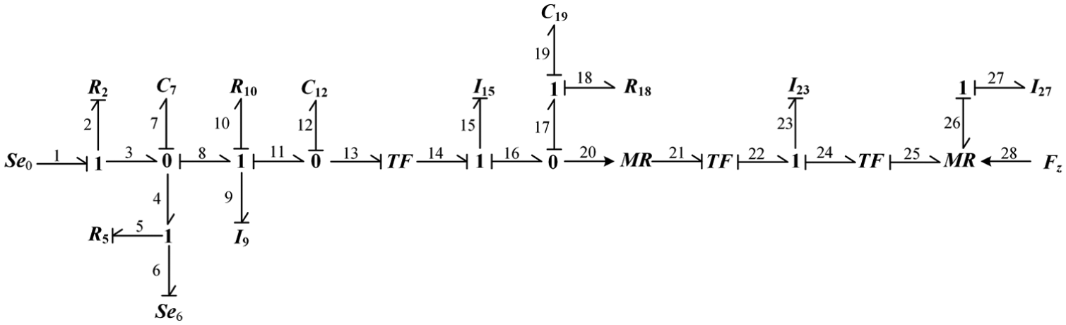
The brake pressure is transmitted into brake force on wheel and finally transmitted into tire brake force to decelerate the vehicle. We consider the brake system and the single-wheel system as an integrated system according to the energy exchange between them. The integrated bond graph model of brake system and single-wheel model is shown in Figure 4.
Integrated model of brake system and single-wheel model.
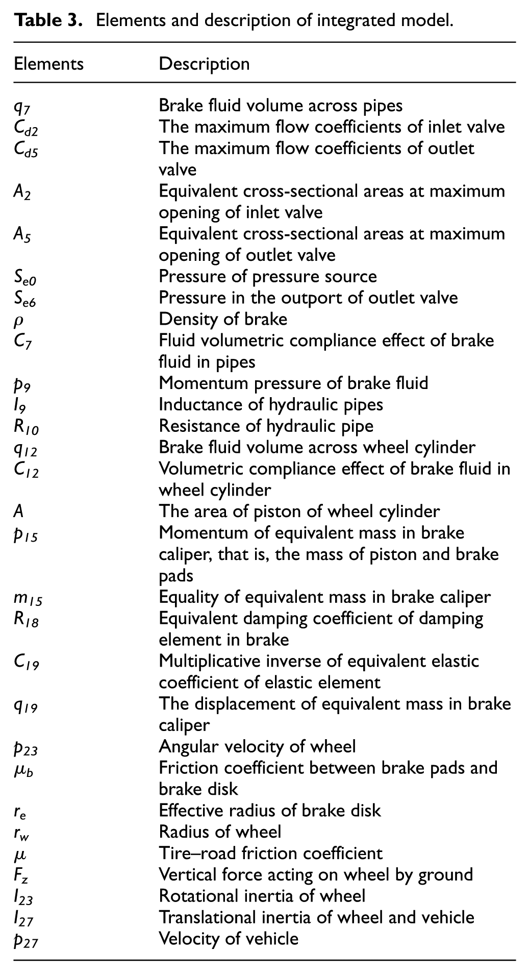
In accordance with the integrated bond graph model in Figure 4, the integrated system states equation can be written. Generalized displacement elements C7, C12, and C19 and generalized momentum elements I9, I15, I23, and I27 are chosen as states variable; thus, the states equation is

The descriptions of elements are demonstrated in Table 3.
Elements and description of integrated model.
Besides, D2 and D5 are the duty ratios of the inlet and outlet valves during building, holding, and dumping cycle of wheel pressure. Their values are between 0 and 1, where 0 means completely closed and 1 means completely opening.
Furthermore, we reset system states

where u1 = D2, u2 = D5, u1 and u2 are the inputs of system (2), x1 is the pressure in port of inlet valve and outlet valve, x2 is the brake fluid flow in hydraulic pipes, x3 is the brake fluid pressure in wheel cylinder, x4 is the speed of piston in brake caliper, x5 is the displacement of piston in brake caliper, x6 is the wheel slip, and Fx is the longitudinal force of wheel.
Model validation
The proposed bond graph model is validated by experimental data for further researching. As the single-wheel model is a commonly used model, only the bond graph brake system model is validated. A hydraulic brake test system shown in Figure 5 is used for brake system model validation. Figure 6 is the structure of experiment system. The test system is made up of an industrial personal computer (IPC), dSPACE simulator, driving circuit system, and hydraulic test module. The hydraulic test module includes normally opened valves 1 and 2; pressure sensors 3, 4, and 5; flow sensor 6; a master cylinder driven by linear motor 7; a HCU; and a brake. The HCU is in X-type arrangement. As the two independent circuits are identical, only one circuit is tested, and the other three ports of another circuit are blocked. The driving circuit system consists of two parts: one for driving solenoid valves and the motor in the HCU and the other for driving testing system solenoid valves 1 and 2 and linear motor 7. A dSPACE simulator is used for real-time simulation, driving valves in the HCU and capturing brake-pressure signals. In the simulator, a DS1005 processor board is used for real-time computing, and a DS2202, DS2211, and DS4003 are used to provide a multi-function signal interfaces.

Brake system test bench.

Structure of experiment system.
The inputs of brake system, including pressure source and inlet and outlet valves control signals, are shown in Figures 7 and 8. In Figure 7, positive value expresses inlet valve signal and negative value expresses outlet valve signal. Wheel cylinder pressures from simulated data of bond graph model and the test system are shown in Figure 8. It is clear that under the same inputs of the brake system, the wheel cylinder pressure simulated by bond graph model is a good fit in with experimental data. In the pressure maintenance stage, the error of simulation data and experimental data is within the range of ±2 bar and the percentage error is within the range of ±4%. As shown in Figure 8, compared with the experimental results, the simulation results have a little delay. Therefore, in the pressure rise and decrease stage, the error is relatively large. However, this process is short. That is to say, the bond graph brake model is accurate and reliable for further usage.

Inlet and outlet valve control signals.
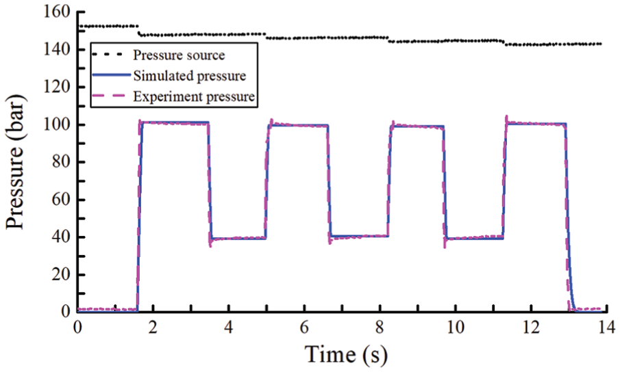
Wheel cylinder pressure validation for test and simulation system.
Sliding-mode controller design
Sliding-mode controller design
First, we rewrite system (2) as follows

where

Step 1
Differential homeomorphic transformation is employed to system (3)
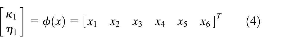
where
Let

and the differential of system (4) is

Then, the transformed systems are shown as follows
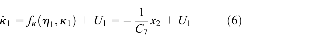

where

Then, the switching function is set as follows

Adopting the exponential reaching law of sliding-mode controller
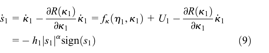
where h1 and α are positive real constant and α is between 0 and 1.
And the input of system (6) is shown as follows

Step i
Differential homeomorphic transformation is employed to reduced system in step i-1
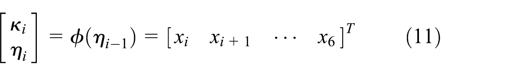
where
We let
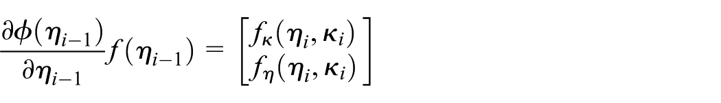
and the differential of system (11) is shown as follows
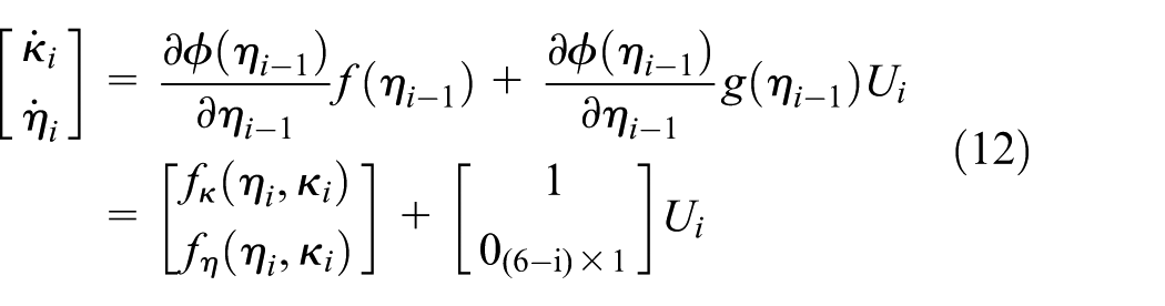


where
Then, the switching function is set as follows

Adopting the index reaching law of sliding-mode controller

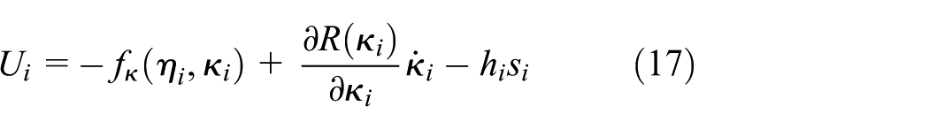
where hi is the positive real constant.
Then, we can get the expression of Ui
Step 6
For the reduced system in step 5, we set switching function as follows

where x6d is the optimal wheel slip ratio.
Adopting the index reaching law of sliding-mode controller

where h6 is the positive real constants.
We can get the expression of U6
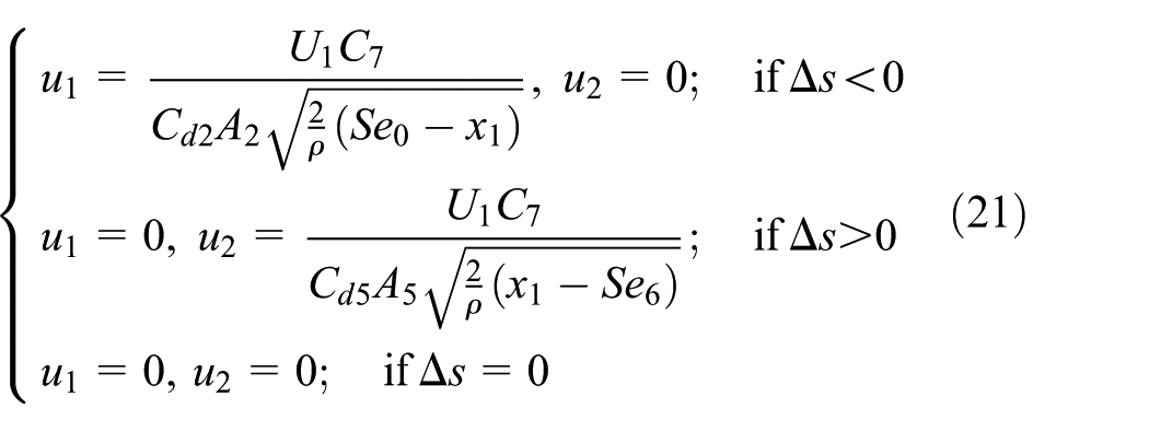
Recalculating the six steps, finally we get the input of system (3), U1. But, U1 is not the input of primal system (2). In primal system, there are two inputs: one is control signal of inlet valve and the other is control signal of outlet valve. However, in brake control, inlet valve and outlet valve are always not open at the same time. In a brake cycle, the working state of the valves can be judged by the change in pressure. Briefly, on pressure building, outlet valve control signal is zero; on pressure damping, inlet valve control signal is zero; and on pressure holding, both inlet valve signal and outlet valve signal are zero.
In this research, an integrated model of brake system and single-wheel system is proposed. As shown in system (2), the only available output is wheel slip ratio rather than wheel cylinder pressure. Fortunately, the change in wheel slip ratio relies upon wheel cylinder pressure. Therefore, slip ratio replaced the wheel pressure as judge signal to get control signals of inlet and outlet valves according to the U1 by sliding-mode controller. By this way, wheel cylinder pressure sensors are not necessary any more, which can save the costs of the system
where
Sliding-mode observer design
In controller design, system state variables feedback should be used. However, in system (2), only wheel slip ratio can be calculated from the measured vehicle speed and wheel speed. Therefore, an observer is necessary to estimate system states.
First, we rewrite system (2) as follows

where
Then, the sliding-mode observer is designed as follows

where

where L is the observer parameter matrix.
The observer error can be obtained by the deviation of system (22) from observer system (23)

To ensure stability of the observer system, Lyapunov stability theory is employed. The following Lyapunov function is chosen

Derivating the Lyapunov function, we can get

It is obvious that the
Estimate of longitudinal force and tire–road friction coefficient
Longitudinal force and tire–road friction coefficient are necessary in the integrated brake–wheel model and the sliding-mode controller. They are estimated according to Zhao et al. 26
Longitudinal force can be estimated as follows


where Cx is the longitudinal stiffness of tire, µ is the tire–road friction coefficient which can be estimated based on recursive least square (RLS) method, 26 s is the wheel slip ratio, and Fz is the vertical force of wheel.
Tire–road friction coefficient is estimated as follows


where

Control strategy parameter analysis
Seven parameters α, h1, h2, h3, h4, h5, and h6 are introduced in the design process of sliding-mode control. In order to ensure the performance of the control strategy, it is necessary to analyze the influence of these parameters. In this article, phase trajectory analysis is used. In the analysis, only one parameter value is changed and the other parameters are fixed, so that the impact of each parameter can be observed clearly. The target slip rate of the wheel is set to 0.12.
The phase trajectory curves of slip rate under different α values are shown in Figure 9. It can be seen from Figure 9 that with the increase in α values, the overshoot of the slip rate gradually decreases, but at the same time, the fluctuation of the slip rate becomes more serious.
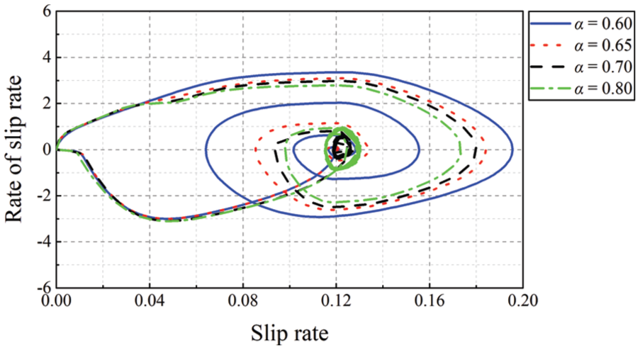
Phase trajectory curve of slip rate under different α values.
The phase trajectory curve of slip rate under different h1, h2, h3, and h4 are shown in Figures 10–13, respectively. From Figures 10–13, it is easy to know that the four parameters have the similar effects on the control strategy performance: with the increase in the parameter value, the stability of the system appears good, but more frequent fluctuations appear near the expectations.
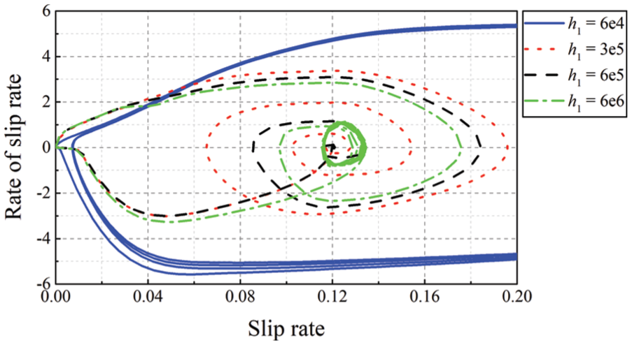
Phase trajectory curve of slip rate under different h1 values.

Phase trajectory curve of slip rate under different h2 values.

Phase trajectory curve of slip rate under different h3 values.

Phase trajectory curve of slip rate under different h4 values.
The phase trajectory curves of the slip rate under different h5 and h6 are shown in Figures 14 and 15, respectively. It is not difficult to find that the parameters h5 and h6 have the similar effects on the control strategy performance: the smaller the value of the parameters, the smaller the change rate of the slip rate and the longer the time of reaching the expected value. However, the larger the value of the parameters, the shorter the time of reaching the expected value, but it will cause the instability of the system.

Phase trajectory curve of slip rate under different h5 values.

Phase trajectory curve of slip rate under different h6 values.
For the control of the wheel slip rate, the response speed is more important and some tiny overshoot are allowed. Therefore, based on the analysis above, the appropriate parameter values selected are shown in Table 4.
Parameter values of the control strategy.

Simulation and analysis
The performance of the proposed brake–wheel integrated controller is verified by simulation. First, MATLAB/Simulink is applied to analyze the responses of sliding-mode controller and integrated model. In order to further verify the actual control effect, MATLAB/Simulink and AMESim co-simulation is applied subsequently, in which brake system is modeled in AMESim environment and sliding-mode controller and observer are built in MATLAB/Simulink environment.
MATLAB/Simulink simulation
To verify controller performance, MATLAB/Simulink software simulation is applied first. The proposed integrated bond graph model, the sliding-mode controller, and the sliding-mode observer are all built in MATLAB/Simulink. The system framework is shown in Figure 16, in which x6 can be found in sliding-mode controller equation (3). The optimal wheel slip ratio is set as 0.12, and the tire–road friction coefficient is set as 0.5. Simulation results are shown in Figures 17–20.

Control structure in MATLAB/Simulink platform.

Wheel slip ratio of Simulink simulation.

Vehicle speed and wheel speed of Simulink simulation.

Inlet and outlet valves control signal of Simulink simulation.

Wheel cylinder pressure of Simulink simulation.
In Figures 17 and 18, it is obvious that the simulated wheel slip ratio converged to optimal value rapidly. At the end of the simulation, the wheel slip reached to 1. It is because that when the vehicle speed is close to zero, the slip ratio will change drastically on small change of wheel speed. Furthermore, the lock of wheels will not result in danger at a pretty low vehicle speed. Thus, in our controller, wheel slip control will quit when the vehicle speed is below 1 m/s. In Figure 17, the vehicle speed is below 1 m/s at about 7.1 s and the controller quitted. Therefore, the wheel locked and the slip ratio increased suddenly. In Figure 19, valves signal value is modulated between −1 and 1. 0 to 1 means inlet valve is under continuous control and the outlet valve is closed, while 0 to −1 means outlet valve is under continuous control and the inlet valve is closed. When the slip ratio is stable, tiny fluctuation of valve signal can be observed, which will be automatically ignored by valve dead zone character. Figures 17 and 20 are the real value and estimated value of wheel slip ratio and wheel cylinder pressure, respectively. It is obvious that estimated values by sliding-mode observer match well with real value and the proposed observer show good performance.
MATLAB/Simulink and AMESim co-simulations
MATLAB/Simulink and AMESim co-simulation system, which is shown in Figure 21, is used to further verify the proposed controller. In this system, the MATLAB/Simulink model is shown in Figure 22 and include S-function, MC pressure, single-wheel model, sliding-mode control (SMC) observer, and controller. The single-channel hydraulic brake system is modeled by AMESim, which is shown in Figure 23.

MATLAB/Simulink and AMESim co-simulation control structure.

Single-wheel, controller, and observer MATLAB/Simulink model.
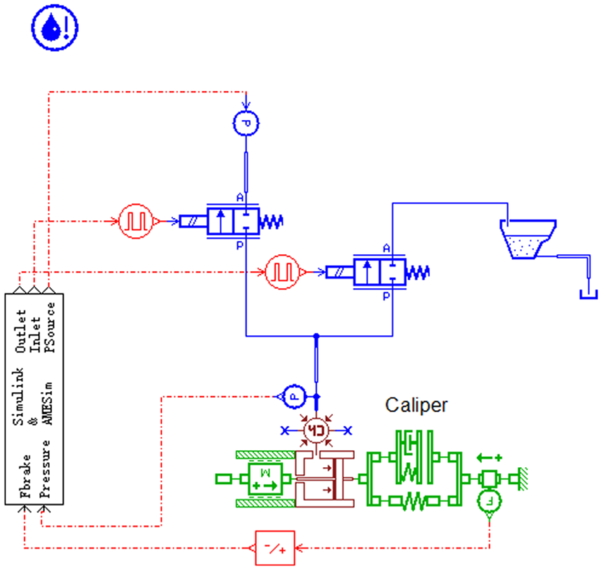
Single-circuit brake system AMESim model.
Vehicles stay stable within a certain slip ratio value, and the highest road adhesion coefficient exists when slip ratio equals a value, and the value is the optimal slip ratio.
Gu and Cheng 27 acquired the optimal slip ratios on three typical roads by experiments, which are 0.08, 0.117, and 0.15 for low-µ, mid-µ, and high-µ roads, respectively. In this study, three typical roads are used for simulation, and their optimal slip ratios are set according to Gu and Cheng. 27
Middle µ road brake
First, mid tire–road friction coefficient (µ = 0.5) is chosen to co-simulation, and the optimal slip ratio is 0.117. Figures 24–26 are the simulation results. Figure 24 shows that wheel slip ratio is modulated to the desired value. As time goes on, the slip ratio increases to some extent, which is because of the vehicle speed reduced with the increase in braking time. Figure 25 is the speed of vehicle and wheel and Figure 26 is the valves control signal.
Wheel slip ratio of mid tire–road friction coefficient.

Vehicle and wheel speed of mid tire–road friction coefficient.

Valve control signal of mid tire–road friction coefficient.
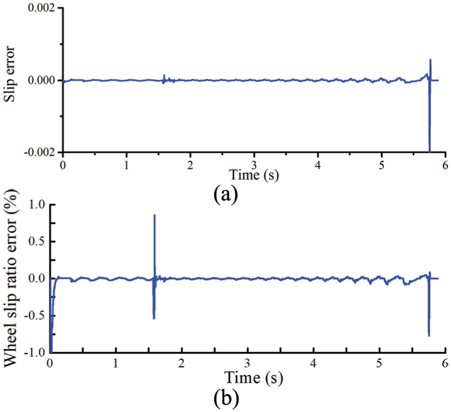
Observer performance is also analyzed. Figure 24 is the wheel slip ratio of real and estimated. It is clear that the estimated slip ratio is closed to its real value. Figure 27 shows the wheel slip ratio error. As shown in Figure 27(a), the error is infinitesimally small. In Figure 27(b), the Y-axis boundary of the coordinate system is set to [−0.1, 0.1]. It is clear that the percentage error is also small, besides the beginning of the simulation. At the beginning, the denominator is small, so the percentage error becomes larger. Although wheel cylinder pressure does not need to be measured in the proposed method, we can use its measured value in AMESim model to analyze estimated value. Figure 28 is the wheel cylinder pressure. It shows that estimated pressure closes to real value. Figure 29(a) presents that the error of real pressure and estimated pressure is within the range of ±2.5 bar. In Figure 29(b), the Y-axis boundary of the coordinate system is set to [−0.2, 0.2]. Figure 29(b) presents that the percentage error is within the range of ±10%, besides the beginning of the simulation. At the beginning, the denominator is small, so the percentage error becomes larger.

Wheel slip ratio error of mid tire-road friction coefficient: (a) wheel slip ratio absolute error and (b) wheel slip ratio percentage error.

Wheel Cylinder pressure of real and estimated in mid tire-road friction coefficient.
Wheel cylinder pressure error of mid tire-road friction coefficient: (a) wheel cylinder pressure absolute error and (b) wheel cylinder pressure percentage error.
Low µ road jump to high µ road
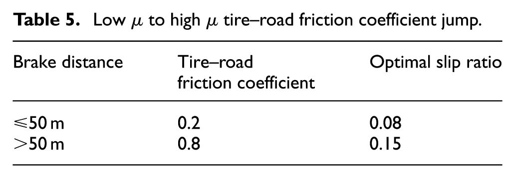
In simulation, the tire–road friction coefficient and the optimal slip ratio are set in Table 5.
Low µ to high µ tire–road friction coefficient jump.
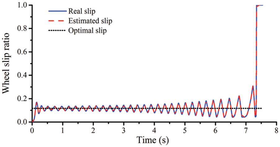
The simulation results are shown in Figures 30–32. Figure 30 shows wheel slip ratio, Figure 31 shows vehicle and wheel speed, and Figure 32 shows valve control signal. It is seen that the wheel slip ratio follows the target value. When the road transient happens, the valve control responds quickly and the slip ratio converges to new target.

Wheel slip ratio in low µ to high µ road jump.

Vehicle and wheel speed in low µ to high µ road jump.

Valve control signal in low µ to high µ road jump.
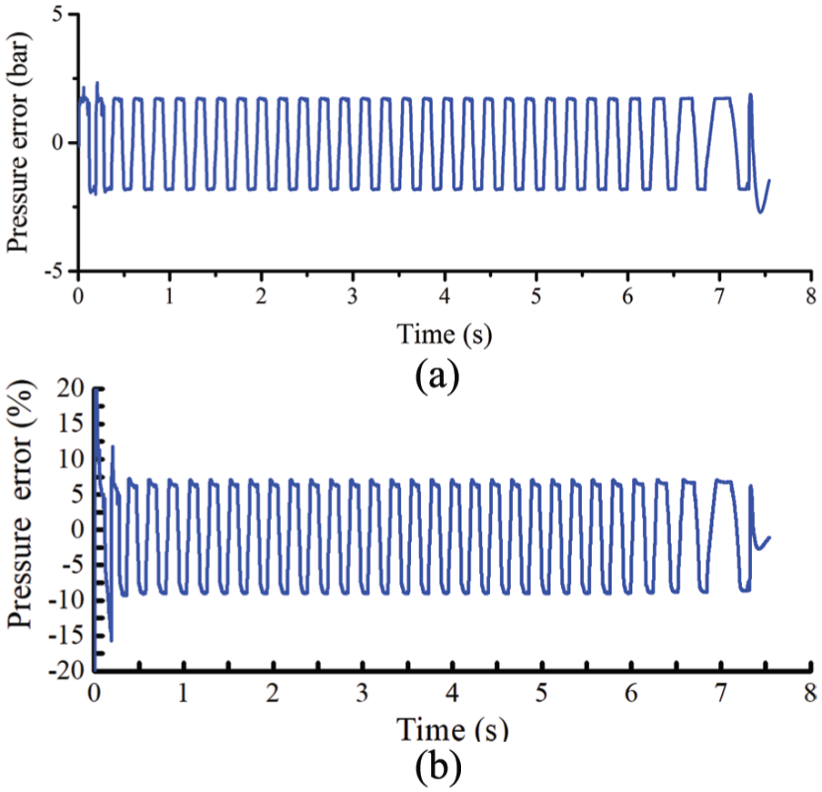
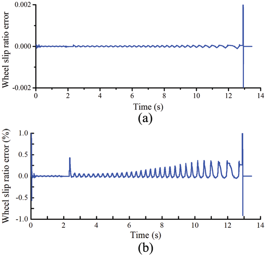
Figures 30 and 33–35 present observer performance. The estimated wheel slip ratio and wheel cylinder pressure are closed to their real values. The error of wheel slip ratio and their percentage error are negligibly small. From Figure 35(a), it is easy to know that the error of wheel cylinder pressure is within the range of ±2.5 bar. As shown in Figures 34 and 35(b), the percentage error of wheel cylinder pressure is larger when the tire–road friction coefficient is 0.2, because the pressure is lower during this time.
Wheel slip ratio error in low µ to high µ road jump: (a) wheel slip ratio absolute error and (b) wheel slip ratio percentage error.

Wheel Cylinder pressure of real and estimated in low µ to high µ road jump.

Wheel cylinder pressure error in low µ to high µ road jump: (a) wheel cylinder pressure absolute error and (b) wheel cylinder pressure percentage error.
High µ road jump to low µ road
Tire–road friction coefficient and optimal wheel slip ratio are set as in Table 6.
High µ to low µ tire-road friction coefficient jump.

Figure 36 is the wheel slip ratio and Figure 37 is the vehicle and wheel speed. Figure 38 is the valve control signal regulated by controller. They show that slip ratio is modulated to desired value. When the tire–road friction coefficient jumps from 0.8 to 0.2, the slip ratio increases inevitably. But it is still modulated to desired value in about 500 ms and the lock of wheel is avoided effectively.

Wheel slip ratio in high µ to low µ road jump.

Vehicle and wheel slip ratio in high µ to low µ road jump.

Valve control signal in high µ to low µ road jump.
Figure 36 presents that estimated wheel slip ratio is close to it real value. And their error is shown in Figure 39. Figure 40 is the real wheel cylinder pressure and estimated value, and in Figure 41(a), it can be seen that the error of real pressure and estimated value within the range of ±2.5 bar except when ABS quits. As shown in Figure 41(b), the percentage error of wheel cylinder pressure is smaller when the tire–road friction coefficient is 0.2, because the pressure is larger during this time, and because of the sudden decrease in pressure, the percentage error has a sudden increased stage.
Wheel slip ratio error in high µ to low µ road jump: (a) wheel slip ratio absolute error and (b) wheel slip ratio percentage error.

Wheel Cylinder pressure of real and estimated in high µ to low µ road jump.

Wheel cylinder pressure error in high µ to low µ road jump: (a) wheel cylinder pressure absolute error and (b) wheel cylinder pressure percentage error.
Conclusion
In most of the present researches of brake system control, hierarchical architectures are widely used, and the layers are designed for vehicle, wheel, and brake system, respectively.
In this article, an integrated model control for mechanical–electronic–hydraulic brake system and single-wheel system is proposed. A nonlinear integrated wheel–brake model is proposed based on bond graph method, and the model is verified by experiment. Based on this model, the nonlinear integrated wheel–brake controller is designed based on sliding-mode method, in which vehicle states are measured by vehicle sensors, and brake system states are estimated by sliding-mode observer. Using this method, brake sensors are no longer necessary, which is valuable in terms of cost savings.
The parameters regulation of the controller is analyzed by phase trajectory method. Then, the performance of the observer and controller is simulated in MATLAB/Simulink and Simulink/AMESim co-simulation, respectively. The results show that the proposed algorithm works well with no brake-pressure feedback.
Footnotes
Handling Editor: Francesco Massi
Declaration of conflicting interests
The author(s) declared no potential conflicts of interest with respect to the research, authorship, and/or publication of this article.
Funding
The author(s) disclosed receipt of the following financial support for the research, authorship, and/or publication of this article: This work is partially supported by National Natural Science Foundation of China (51775235, 51575225), Jilin Province Science and Technology Development Plan Projects (20180201056GX), and Science and Technology Project of Department of Education of Jilin Province (JJKH20180077KJ).