Sage Journals: Discover world-class research

Abstract

This article presents a simulation program for previewing and emulating three-dimensional printing. The proposed simulator adopts a voxel-based virtual manufacturing approach to fabricate the target model in a virtual volume space. A mass-diffusion procedure coupling with adaptive filament deposition is used to generate the printing roads of the virtual manufacturing model. Thus, the resultant virtual model resembles the printed object better. As the virtual model has been built, the simulator performs line-drawing, animation and volume rendering to reveal the progression of the printing and the geometric features of the model, including its outer appearance, surface roughness and internal structures. Hence, more geometrical features of the model are shown. During the virtual manufacturing process, semantic error checking is also carried out to detect potential printing errors which may cause supporting problems, collisions, over- and under-extrusion, and other printing failures. Two efficient algorithms, using three rasters of voxels, are developed to conduct the kernel computations such that the run-time semantic error checking is simplified and the memory usage is reduced. Equipped with advanced modelling, debugging and graphics techniques, the proposed simulator can be used as a virtual three-dimensional printer as well as a debugger in additive manufacturing procedures. Users can utilize it to preview the resultant model and to evaluate the printing process such that potential errors can be prevented and the quality of the printed parts can be enhanced.

Keywords

Three-dimensional printing virtual manufacturing simulation volume rendering

Introduction

Three-dimensional (3D) printing techniques are widely used for prototyping and manufacturing. In a 3D printing process, the fabrication procedure is driven by a G-code program which comprises with printing commands and parameter setting instructions. If syntax and semantic errors exist within these machine codes, the process will encounter failures which delay the manufacture schedule and increase the costs. In some extreme cases, the printer would be damaged if these errors are fatal. Three commonly seen printing errors are shown in Figure 1. These errors were not detected by examining the G-codes, but they showed up in the printed objects. Therefore, the users need tools for previewing the printing processes and resultant models such that they could find and correct these errors in advance.

Figure 1.

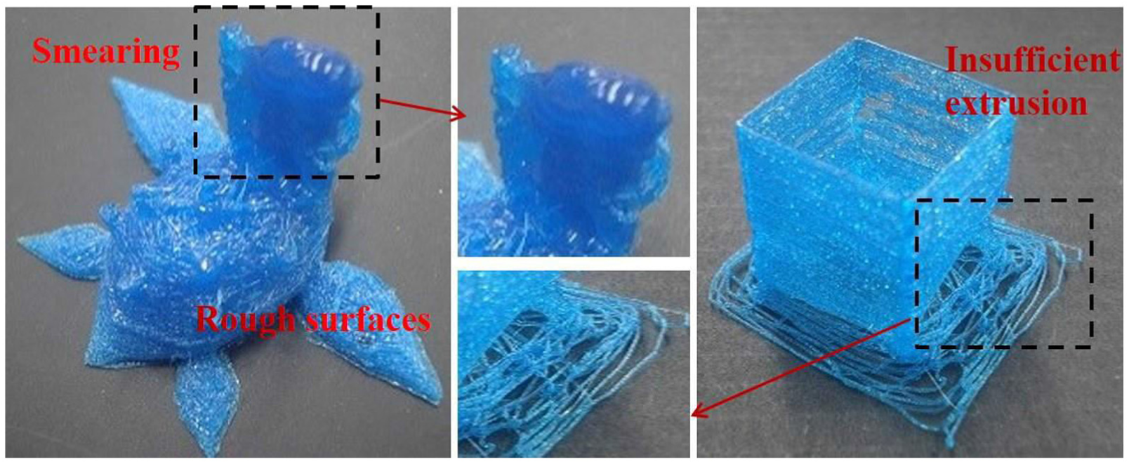
Three commonly seen printing problems: smearing, rough surface and broken surface caused by improper printing actions.

Choi and Chan¹ proposed two simulation procedures for previewing powder-based and layer-based prototyping. Jee and Sachs² developed a simulation procedure for metal-powder-based layer manufacturing. Ferreira³ integrated modelling, surface rendering and related techniques with rapid prototyping to reduce printing errors. A simulator should be developed according to experimental and theoretical models of the target system. Some testing results, mathematical models and approximation approaches for 3D printing had been published. Anitha et al.⁴ conducted several experiments and used Taguchi technique to figure out influential parameters in 3D printing. They found that the layer thickness is the most crucial one.

Chandru et al. proposed a voxel-based modelling computer-aided design (CAD) system for creating and previewing models for rapid prototyping using voxels.⁵ A similar work was presented in Aremu et al.⁶ The authors designed a CAD tool using lattice structures to model objects aiming for additive manufacturing. Skin surface formation and structure strength of the target objects were also discussed in the article. A recent review article about additive manufacturing methods and the related mathematical models were published in Bikas et al.⁷ This article also discussed the validation of these models and suggested that more accurate models should be created to assist additive manufacturing.

Among all 3D printing machines, fused deposition modelling (FDM) printers hold the largest market share in terms of the number of installations.⁸ Thus many research results on modelling FDM processes had been presented. In the literature,^1,9,10 thorough studies on FDM printing and the influential parameters were reported. The authors also proposed mathematical formula to model both the control mechanisms and the typical characteristics of FDM printers. Feed rate and filament extrusion play important roles on the quality of the finished parts. A test was conducted to study the effects of feed rate on filament flow by Ibrahim et al.¹¹ The influences of nozzle temperature and material on FDM printing were also reported in the same article.

Some physical simulators had been created on the purposes of previewing G-code programs.^12,13 These simulators can be downloaded or invoked from the Internet and have become popular G-code previewers for 3D printing hobbyists. These simulators use lines to approximate the printing roads and animate line-drawing to visualize the printing process. Since the target model is modelled using lines, surface roughness, filling patterns and internal structures of the model are not revealed by these simulation tools. Their previewing functions are primitive and should be significantly expanded. These simulators check syntax errors of the input G-code programs. However, they perform very limited or no semantic error checking Infeasible and dangerous printing actions are not figured out. Ueng et al.¹⁴ improved 3D printing simulation by incorporating more sophisticated graphics and error checking techniques into their G-code interpreter such that the results were more comprehensible and the fidelity of the resultant virtual object was improved. Nonetheless, more work should be done to enhance the capabilities of their simulator in debugging the G-code program and fabricating the virtual model.

In this article, we propose a powerful simulator for FDM 3D printing. The simulator interprets the input G-code program and builds a virtual model in a volume space step by step to emulate the progression of the 3D printing. The mathematical models presented in the literature^1,9,10 for modelling FDM printers are adopted in the creation of the simulator such that the basic functionalities of traditional G-code simulators^12–14 are supported. The system also comprises more advanced modelling techniques, including a diffusion model and a deposition function of filament, to generate printing roads in the volume space. Consequently, the fidelity of the resultant virtual model is well enhanced, compared with the line-drawing methods.^12,13 The proposed system utilizes volume visualization and animation techniques to display the resultant model and to reveal the progression of the 3D printing. More geometrical features of the 3D model can be shown. To prevent printing errors, the simulator detects not only syntax errors but also semantic errors hidden in the G-code program and offers debugging information to the users. Hence, the users can discover illogical printing actions earlier and avoid manufacturing failures in the model production stage.

System overview

The proposed simulator is dedicated to FDM process which is widely used because of lower operational costs and cheaper installation fees.⁸ In an FDM process, the printer manufactures the target model in a line-by-line and layer-by-layer manner. To print a line, called a road in the literature,^9,10,14 the printer pushes filament into a hot chamber where the filament is melted. Then, it extrudes the melt along the path specified by the G-code. Once printed, the road is cooled and solidified in a short time period. After completing the fabrication of a layer, the printer lowers the printing bed or raises the nozzle by a distance equal to the thickness of the layer and starts to print another layer.

Since the proposed simulator focuses on FDM process, it will operate in a specific way which virtually resembles the FDM-layered manufacturing process. An overview of the simulation procedure is given in this section while detailed descriptions of the kernel procedures and data structures will be presented in the following sections.

The simulation program is operated according to the flowchart shown in Figure 2. The simulator fetches the input G-code program from a disc file. Then, it performs basic syntax and semantic error checking to ensure that the G-codes are free from incorrect instruction formats and infeasible parameter settings. For example, the nozzle temperature should be set within a predefined range and the nozzle should move inside the allowable space of the 3D printer. Besides detecting basic errors, the simulator creates a data structure, the G-code table, which will be used in following simulation steps to manufacture the virtual model and to detect illogical printing actions. Then, the simulator interprets the G-codes to set printing parameters and creates a virtual volume space for conducting the remaining simulation steps.

Figure 2.

Flowchart of the proposed simulation procedure.

After completing the preparation tasks, the simulator starts to fabricate the virtual manufacturing (VM) model in the volume space. The resultant VM model will be stored in a disc file. While building the VM model, the simulator also conducts run-time semantic error checking to detect potential printing problems, including un-supporting parts, overlapped printings, collisions and so on. To offer the users debugging information, the segments of the G-code program containing these errors are retrieved from the G-code table and displayed in a window of the user interface.

At the final stage of the simulation, volume rendering and related graphic techniques are employed to explore the geometric features of the VM model, including surface roughness, filling patterns and internal structures, which are invisible using conventional simulation methods.

VM process

The VM process is one of the major procedures of the simulation. Both the VM model fabrication and the semantic error checking are performed in this process. In this section, the creation of the volume space and the G-code table and the fabrication method of the VM model are presented. Semantic error checking is described in the next section.

The G-code table

At the pre-processing stage, the G-codes are browsed and divided into groups. Each group of the G-codes are responsible for building a layer of the VM model and are recorded in a linked list. Each node of the linked list keeps the original G-code instruction, line-number of the instruction, filament extrusion length, feed rate and positions of the two ends of the road. Then, these G-code nodes are sorted according to their line numbers, and the resultant linked list is stored in the G-code table, which is shown in Figure 3. The G-code table contains N entries, where N is the number of layers to be built. Each table entry contains pointers to the head and tail of the associated linked list and the essential information about the corresponding layer of the VM model, including the thickness and z-coordinate of the layer.

Figure 3.

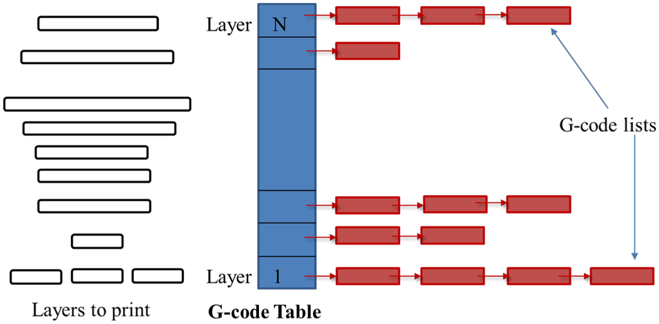
The G-code table and the associated layered manufacturing.

The G-code table is one of the major data structures in the VM process. When fabricating a layer of the VM model, the corresponding linked list containing the G-codes is retrieved from the G-code table, and the G-codes are then interpreted to construct the layer. If errors are detected in the VM manufacturing, the responsible G-codes can be identified, based on the recorded information in these G-code nodes. The G-code table is also utilized in the visualization process for displaying the toolpaths, animating printing progression and locating the correspondent G-codes. To accomplish these goals, the users select the G-codes building the target layers from the G-code table via a graphical user interface (GUI) first. Then, the progression of the printing process is shown using line-drawing animation techniques such that the toolpath planning, printing speed and outer shape of the VM model are revealed.

The volume space and voxel-based VM modelling

In conventional G-code simulators, the VM model is built using lines or rectangular bars. The resultant virtual model is a poor approximation of the physical model. Its shape is fuzzy and its internal structures and filling patterns are occluded by its exterior surface. Thus, users gain limited knowledge about the geometric features of the VM model. In the proposed simulation method, we build the VM model using voxels which are rectangular cubes of a fixed shape and size to improve the fidelity of the VM model. The voxel-based modelling approach also enables users to explore the geometric features of the VM model using volume rendering techniques in the visualization stage of the simulation. Furthermore, it greatly simplifies the semantic error checking by cross-referencing adjacent layers of the VM model. A voxel-based model is shown in Figure 4. The left image displays the original polygon-based model, and the right image shows the voxel-based model.

Figure 4.

An example of voxel-based modelling – left: a polygon-based model, right: the voxel-based model.

To create the volume space, we compute the bounding box (BB) of the target model at first. Then, we enlarge the BB slightly to accommodate the expansion of the printed roads and the swelling of the VM model. At the following step, the BB is split into voxels, based on a regular grid. The resolution of the grid should be higher than the resolution of the physical printer. Thus, the shape of a road can be better approximated in the volume space.

VM process using a three-raster approach

In the concept, the VM model is built in the volume space using voxels. In order to achieve a better geometrical accuracy, the resolution of the embedded grid must be high. Therefore, the required memory space would be large. If the memory of the computer is limited, the VM process will encounter difficulties. In order to overcome this problem, we develop an innovative approach to manufacture the model in the volume space using less memory.

In the approach, instead of creating the whole volume space, only three layers of voxels are created. These rasters are associated with different duties in the VM process. The arrangement and usage of these rasters are depicted in Figure 5. The middle raster is used to create the current layer. The manufacturing results of the previous layer are recorded in the lower raster. Sometimes, the nozzle may extrude too much filament in building a road and causes over-extrusion of filament. Thus, some voxels of the road contain excessive filament, and their heights are larger than the thickness of the current layer. If so, the filament overflow is removed from the middle raster and then stored in the upper raster. However, if under-extrusion occurred in fabricating the previous layer, some voxels of the lower raster were not fully filled. Their heights are less than the specified layer thickness. To compensate the under-extrusion and to reflect this phenomenon, the simulator moves filament from the voxels of the middle raster, which are vertically above and filled with filament, into these partially filled voxels of the lower raster.

Figure 5.

Three rasters are used in the VM process; the current layer is created in the middle raster; the previous layer is stored in the lower raster; the upper raster holds the overflow of filament from the middle raster.

As the current layer has been built, the contents of the lower raster are output to a disc file. Then, the roles of these three rasters are cycled. The middle raster is regarded as the new lower raster and the lower raster is designated as the new upper raster. The upper raster is treated as the new middle raster. Since the upper raster contains filament overflow from the middle raster, the next layer of the VM model will be built on top of the current layer and the filament overflow. Therefore, over-extrusion is accumulated. However, if under-extrusion happened in building the current layer, the partially filled voxels will be compensated when the next layer is manufactured.

As the costs of hardware are getting cheaper, the computer is usually equipped with large memory space and the entire volume space can be created. Under such situation, the three-raster approach is still applicable. However, no raster-cycling is necessary and the VM model is not output to the disc file until the entire VM process has been completed.

Deposition of filament

In conventional simulation methods, printed roads are represented by lines, rectangle bars or other geometries with regular shapes.^1,12–14 However, in the work of Jee and Sachs² and Turner and colleagues,^9,10 it had been proved that the shape of a road is not regular. When printing a road, the 3D printer deposits more filament at the two ends and extrudes less filament at the middle section. This is caused by the acceleration of the nozzle at the beginning of the printing and the deceleration of the nozzle at the end of the printing. Thus, as the road solidifies, its shape looks like a bar with varying cross-sections, as shown in Figure 6. In this work, we invent a method to emulate road-printing of FDM process. The method consists of two stages. At the first stage, a line of unit-width is drawn in the middle raster and filament is deposited into the voxels of the line according a deposition function. At the second stage, a diffusion process is performed to transport the filament to the adjacent voxels to form a bar of irregular shape.

Figure 6.

(a) Deposition functions of different feed rates, (b) deposition function of various road lengths and (c) shapes of long and short road.

The line of unit-width is rasterized in the middle raster using Bresenham’s algorithm.¹⁵ The total volume of the filament of the road is computed by decoding the G-code. Then, based on one of the deposition functions shown in Figure 6(a) and (b), filament is deposited to the voxels covered by the line. We classify the deposition of filament into several cases according to the road length and the feed rate. When printing a long road, the filament extrusion pattern is decided by the feed rate as shown in Figure 6(a). If the feed rate is high, the acceleration and deceleration are significant. Thus, more filament is deposited at the two ends. However, if the feed rate is low, the filament deposition is more uniform. In case that the road is short, the acceleration and deceleration of the nozzle dominate the filament deposition. Thus, more filament is deposited in the road, and this short road becomes a bump, as shown in Figure 6(b).

Diffusion process of filament

Once the filament has been distributed over the voxels of the line, a diffusion process is triggered to transport the filament to the adjacent voxels. The diffusion process is modelled as follows

\frac{\partial M (x, y, t)}{\partial t} = D (x, y, t) \nabla^{2} M (x, y, t)

(1)

where M is the volume of filament at position (x, y) at time t, and D is the diffusion coefficient. The diffusion coefficient is determined by two functions and defined as

D (x, y, t) = K (t) * H (‖ \nabla^{2} M ‖)

(2)

where K(t) decays with time t and is approximated by

K (t) = {\begin{matrix} 1, & 0 \leq t \leq 3 Δ t \\ \exp ((- t / Δ t) + 3), & 3 Δ t < t \leq 6 Δ t \\ 0, & t > 6 Δ t \end{matrix}

(3)

where Δt is the time step size of the numerical solver of equation (1). We use K(t) to control the diffusion time such that the diffusion of filament will be completed within a few time steps to manifest the quick cooling and solidification of the road. The function H(.) is defined as

H (‖ \nabla^{2} M ‖) = {\begin{matrix} 0.333, & ‖ \nabla^{2} M ‖ \geq c \\ 0, & ‖ \nabla^{2} M ‖ < c \end{matrix}

(4)

Equation (1) is solved using a finite difference method. The middle raster is the problem domain. Its voxels constitute the underlying grid. All computations are carried out in this grid. No matrix is formed. Since K(t) becomes zero after a few iterations, the computation will definitely converge.

The rationale behind our filament diffusion model can be explained as follows: as the melted filament leaves the nozzle, it is a hot and viscous liquid and flows to the surrounding area if the filament volume is low there. We use M to represent the volume of filament at position (x, y) at time t. Initially, M is equal to the filament volume extruded by the nozzle. The Laplacian represents the difference between the filament volume of the point (x, y) and the average filament volume of the surrounding area. If the magnitude of the Laplacian is greater than a threshold c, then there is a filament flow into or out of the voxel. However, if the Laplacian magnitude is smaller, the local distribution of filament is relatively uniform and there is no mass-transport. The function H(.) is used to act as the switch of the filament flow and to set a threshold for the flow rate such that the flow can happen only under a certain condition, and the portion of filament flowing into or out of the voxel is limited. The value of c is equal to one half of a voxel’s volume and the value of H(.) is set to 0.333 based on experimental results. As time elapses, the filament solidifies as its temperature decreases and no filament flow is possible. To reflect this cooling effect and the reduction of diffusivity, function K(t) is employed to model the decay of diffusivity because of the cooling effect. The graph of K(t) is shown in Figure (7). At the first three time steps, the temperature of the melted filament is hot and the diffusivity is active, and hence, the value of K(t) is set to 1. Then, its value exponentially decays in the following three steps to reflect the cooling and solidification of the deposited filament. As the time elapses, the filament solidifies and the diffusivity stops. Therefore, K(t) is set to 0.

Figure 7.

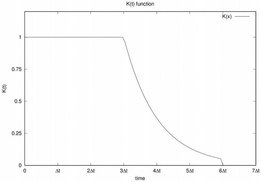
The diffusivity process of the extruded filament is controlled by the K(t) function. The graph shows the three stages of diffusivity, the active, exponential decay and non-diffuse stages.

Run-time semantic error checking

The run-time semantic error checking is performed along with the fabrication of the VM model. When creating a layer, the following potential problems are detected: unsupported parts, collisions, smearing, short cooling time, over- and under-extrusion, and overlapping. The detection of these infeasible printing actions is achieved by examining the contents of the three rasters as shown in Figure 8.

Figure 8.

Run-time semantic error checking using three rasters: (a) unsupported part detection, (b) over-extrusion and (c) collision and smearing.

Unsupported parts

A newly created road will collapse if any one of the following two situations occurs: (1) It is not supported under the two ends. (2) Both the ends are supported, but some segments of the road are long and unsupported. To detect the first situation, the simulator examines the voxels in the lower raster, which are vertically below the two ends. If any of these voxels are empty, the road may collapse on one or both ends and the simulator sends a warning message to the users. To check the second situation, the simulator computes the lengths of the unsupported segments of the road first. If an unsupported segment is longer than a threshold, the simulator issues a warning message. We conducted numerous experiments and found out that the threshold is about 4 cm for FDM printing. The detection of unsupported parts is illustrated in Figure 8(a).

Improper extrusion detection

To find over- and under-extrusion, the volume of extrusion is calculated from the G-code instruction and is compared with the volume of the printed road. If a significant difference is detected, a warning message is issued. On some occasions, the extrusion is normal but the toolpaths are not well scheduled. Hence, the roads mutually intersect and create filament overflow in the intersection points. This phenomenon is very common when filling a solid model. Its influence is usually mild but may cause problems in the future printing, if the filament at the intersection points is getting larger. In our simulator, those voxels which are printed by multiple G-codes are figured out and their filament volumes are examined to avoid overflow in future printing actions. This situation is depicted in Figure 8(b). Over extrusions usually happen at the intersections of roads. The surplus of the filament is moved to the upper raster.

Collision and smearing detection

When the height of the accumulated filament exceeds the layer thickness, the nozzle may collide with the accumulated filament and melts it as well as the part beneath. Thus, previously printed parts will be damaged and the current layer cannot be built either. This phenomenon is shown in Figure 8(c). In the runtime the accumulated filament in the upper raster is monitored. Once its height exceeds the layer thickness, a warning is reported such that the users can be aware of this error and figure out the responsible G-codes.

Insufficient cooling time

When a layer of the model has been printed, it needs time to cool down and solidify. If the inter-layer-printing time is too short, the new layer may melt the previously printed layer and causes damages to the model. To prevent such an error, the time of printing a layer is computed. If the printing time is less than a threshold, a warning message is sent to the users and suggests the users to insert a waiting instruction in the G-code program to pause the printer for a while to avoid the over-heating problem. This threshold of cooling time is related to the room temperature. Based on our experiences, the inter-layer-printing time should exceed 1.7 s when the room temperature is about 26°C.

Three types of instructions affect the printing time of a layer. They are the motion (or printing) instructions, the pausing instructions and the heating instructions. We assume that the nozzle is heated at the initial stage. It is unnecessary to heat the nozzle again when printing a layer. Thus, our simulator neglects the heating time when computing the printing time of a layer. It accumulates only the elapsing time of motion and pausing instructions to obtain the printing time of a layer. The motion of the nozzle is controlled by G0 and G1 instructions. For each motion instruction, the simulator calculates the moving distance of the instruction at first. Then, the distance is divided by the current feed rate to obtain the elapsing time of the instruction. The feed rate represents the moving speed of the nozzle and is usually encoded in the motion instruction. The pausing of the nozzle is controlled by G4 instructions. The pausing time of a G4 instruction is specified in the operand field and can be directly obtained from the instruction.

Visualization method

Two major visualization methods are employed to preview and evaluate the 3D printing process. In the first visualization technique, volume rendering is used to reveal the surface roughness, appearance, internal structures and filling patterns of the VM model. The second visualization method utilizes animation and line-drawing to show toolpaths and the progression of the printing.

Volume visualization

The flowchart of the volume visualization is shown in Figure 9. At first, the volume field M(x, y, z) produced in the VM process is fetched into the main memory from the disc file. Then, the gradient field of M(x, y, z) is computed. The directional vectors of the gradient at all the voxels are utilized to build a 3D texture, which will be used to calculate the normal vectors in the volume rendering process such that VM model can be shaded. Besides, the histograms of the gradient magnitude and the intensity of M(x, y, z) are shown in a window of the GUI. According to these two histograms, the user creates a two-dimensional (2D) transfer function to assign colours and opacities to the voxels. The transfer function is then converted into a 2D texture which is employed to interpolate pixel colours in the volume rendering process. Once the pre-processing stage has been completed, the 2D and 3D textures are moved to the graphics processing unit (GPU). Then, a hardware-accelerated slicing method is used to render the VM model. In the rendering method, the data volume is cut into consecutive view-aligned slices which are perpendicular to the view direction. These slices are texture mapped with the 2D and 3D textures such that the colours, opacities and normal vectors of the pixels can be computed. Then each slice is rendered using Phong shading method, and the rendering results of all slices are blended in the back-to-front order to form the final volume rendering image. Since the rendering, shading, texture mapping and blending computations are assisted by the GPU, the volume visualization can be carried out in realtime.¹⁶

Figure 9.

The flowchart of the volume visualization procedure.

Some advanced functionalities are supported in our volume visualization procedure such that the user can explore the VM model in various aspects. For example, the users can modify the transfer function to give high opacities to the voxels in the VM model’s boundaries such that the appearance and surface roughness of the VM model are shown. The users can also use the gradient directions and magnitudes to tune the opacities of the voxels to enhance the boundaries or to produce see-through effects in the volume rendering In order to reveal the internal structures and the filling patterns, the users can remove some parts of the model using a cutting plane.

Printing progression visualization

The toolpaths and printing progression are displayed layer by layer and line by line. Before rendering the toolpaths of an individual layer, the associated linked list of the G-codes is retrieved from the G-code table. Then, these G-codes are interpreted one after another to produce the printing roads. These roads are represented by transparent and shaded lines, and the whole printing progression is animated in realtime such that the users can understand how the VM model is built. The users can also modify the opacities of the lines to view the internal parts or the outer shape of the VM model. In order to give the users better knowledge about the VM model and the toolpaths, the animation is created in four different angles and using both parallel and perspective projections.

The users can chose a suitable angle to view the animation. They can also visualize the printing process in the four angles at the same time.

Experimental results

Experiments have been conducted to verify the capabilities of the proposed simulator. Some test results and comparisons are presented in this section. The 3D geometry models used in these tests include an open box, a conic tower, a comb, a mushroom, a Sphynx and a Lapras model. The STL files of these models are processed using a commercial slicer to generate the G-code programs. Then, the G-code programs are emulated by the proposed simulator and two conventional simulators to produce the VM models. Some of the G-code programs are sent to an FDM 3D printer to fabricate physical models such that the fidelity of the VM models can be visually evaluated. The proposed simulator is implemented using OpenGL shading language and C-language without using other graphical libraries.

Comparison with conventional simulators

The simulation results of the Sphynx model are displayed in Figures 10 and 11. In Figure 10, some simulation results using our simulator are shown. In Figure 10(a), the line-based VM model is displayed. It is created by the visualization procedure to show the printing progression and toolpaths. The opacities of the lines of the Sphynx are small while the opacities of the lines of the base are larger. Thus, the base is clearly displayed. In Figure 10(b), the voxel-based VM model is drawn using the volume rendering procedure. The boundary voxels of the VM model are given high opacities. Then, the whole model is rendered with shading effects to reveal the appearance and surface roughness of the model. Figure 10(c) is also produced by the volume visualization procedure. The opacities of the voxels are adaptively adjusted according their gradient directions such that the model surface facing the viewer is removed. In consequence, the Sphynx becomes transparent and the internal structures and filling patterns of the base are displayed. For comparison, the physical model fabricated by the 3D printer is given Figure 10(d). Comparing Figure 10(b) and (d), the VM model created by the proposed simulator highly resembles the physical model.

Figure 10.

Simulation results using the proposed simulator are shown in (a) line-based model, (b) voxel-based model and (c) internal structure. For comparison, the printed model is displayed in (d).

Figure 11.

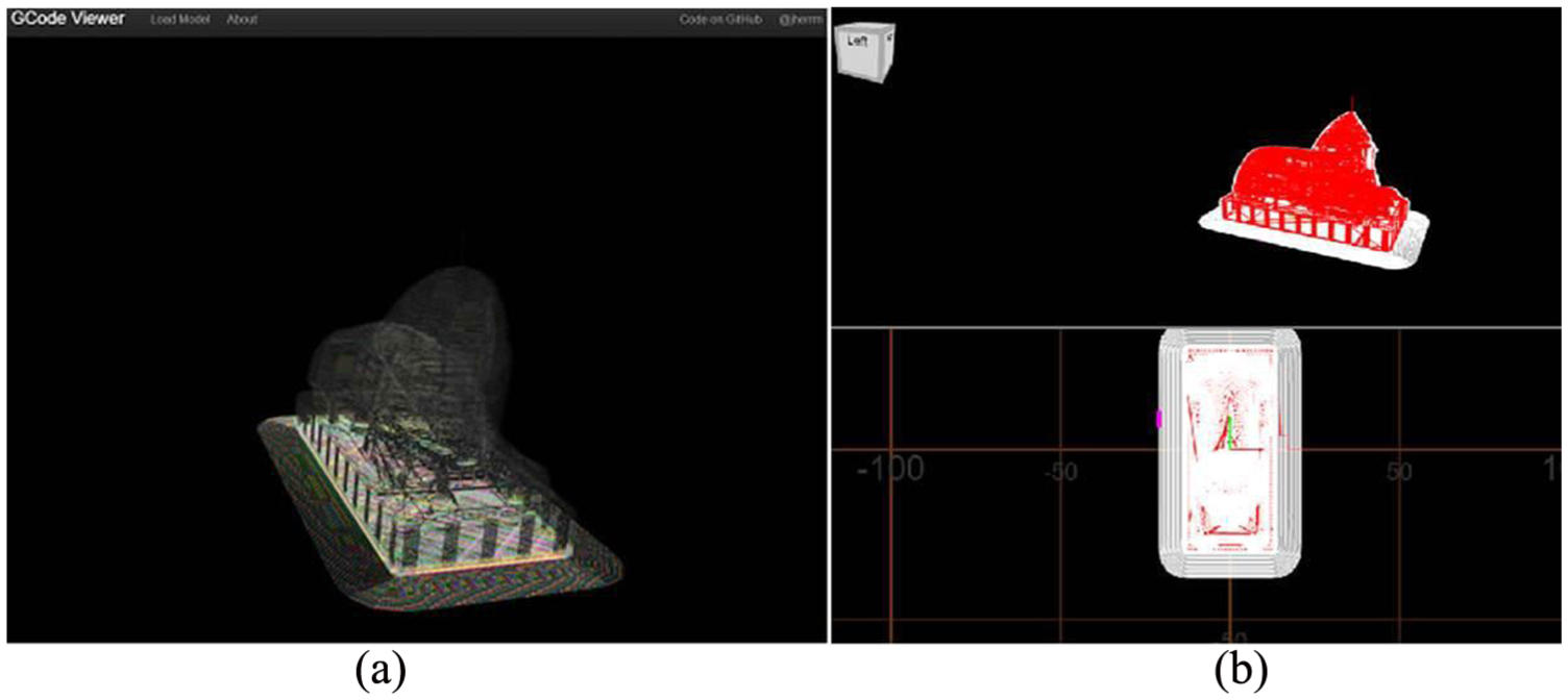
Simulation results of two conventional simulators: (a) simulation result of system 1 and (b) simulation result of system 2.

The simulation results using the G-code interpreters, G-Code Q’n’dirty Toolpath Simulator¹² and G-code Viewer¹³ are shown in Figure 11. In these two simulators, toolpaths are displayed using line-drawing and animation techniques. Users can view the animation in different angles. However, the target model is poorly approximated by the line-based models. Furthermore, the model is not shaded, and thus, the shape and surface roughness are hardly understood. Since the lines are opaque, the internal structures and filing patterns are occluded and limited geometric features are revealed in the results.

For the purposes of comparison with these two conventional G-code simulators, a snapshot of a simulation process conducted using the proposed simulator is shown in Figure 12. In the simulation, the proposed simulator builds the VM model, a mushroom, using shaded lines. Thus, the shape and surface roughness of the VM model are better illustrated. Our simulator also possesses a better GUI. It renders the VM model in the main window and displays the correspondent G-codes in upper left window. The bottom of the left window contains a menu which allows the users to tune the optical parameters and display modes of the visualization procedure. Other functionalities of the proposed simulator can be triggered by the menu buttons shown in the right column of the GUI.

Figure 12.

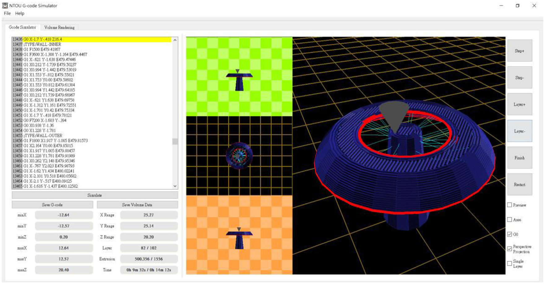
VM model fabricated using shaded lines and the GUI of the proposed simulator.

G-code revision using simulation results

Originally, the box and the Lapras models couldn’t be fabricated by the 3D printer. The errors are shown in Figure 1. The failure in printing the box is caused by under-extrusion. The feed rate is too fast and the filament deposition is too low in the middle sections of the roads. Using the proposed simulator, we find the responsible G-codes. Then, we slow the feed rate and increase the extrusion lengths of filament of the G-codes. Then, the revised G-code program is emulated by the proposed simulator. The simulation result and the printed model are shown in Figure 13(a). The surface quality of the physical model is significant improved, though it can be enhanced further.

Figure 13.

Simulation and printing results using revised G-code programs: (a) Box – left: simulated, right: printed and (b) Lapras – left: simulated, right: printed.

The body of the Lapras model could be successfully printed. However, smearing occurred when the printer tried to fabricate the neck, as shown in Figure 1. Based on simulation results, we found that the road lengths of the neck are short and too much filament was extruded when the roads were printed. Thus, the nozzle collided with the accumulated filament and melted the neck. We utilize the toolpath animation module and the semantic error checking module of the proposed simulator to find the G-codes manufacturing the neck. Then, the filament extrusion of the G-codes is reduced and the target model becomes printable. The simulation and the printed results of the revised G-code program are shown in Figure 13(b).

The printing progression visualization

The animation of toolpaths is a traditional technique in G-code previewing process. We enhance this technology by offering more view directions and using a better line-drawing method. First, the animation is displayed in three orthographical view angles using parallel projection and in a user-defined angle using perspective projection. Therefore, users can see the simulation results via different angles. Second, in order to reveal the size of the VM model, grid lines and checkerboard patterns are drawn in the background of the images. Third, the user can change the opacities and colours of the lines to reveal inner parts of the VM model via the GUI as displayed in Figure 12. A snapshot of the animation of printing the Sphynx model is shown in Figure 14. In the images, the model is created using transparent lines without shading effect.

Figure 14.

Animation of the printing process and toolpath rendering.

Semantic error detection

Run-time semantic error checking is one of the major functionalities of the proposed simulator. Three examples of semantic error detection are presented and discussed in this section. First, the example of discovering unsupported printing is depicted in Figure 15. In this simulation, the G-codes for building the mushroom model are emulated. Our simulator found no error when virtually manufactured the stalk. However, it discovered unsupported printing errors as it tried to build the cap. The unsupported layer of the model is shaded with red colour and the correspondent G-codes are retrieved from the G-code table and highlighted with red colour, as shown in the left part of this figure.

Figure 15.

Semantic error detection reveals unsupported parts.

Inter-layer cooling time plays an important role in 3D printing, though it had seldom discussed in the literature. In our simulator, the inter-layer cooling time is examined after manufacturing a layer. If it is less than a predefined threshold, a warning message will be issued. An example is illustrated in Figure 16 to demonstrate the detection of an insufficient cooling time. In the left image, a snapshot of the simulation is presented. It shows the layers built without sufficient cooling time and the correspondent G-codes in yellow colour. The printed model, a conic tower, is shown in the right image. The image reveals that the top layers of the tower are twisted because of insufficient cooling time. Since these layers are relatively small, they are built in short time interval and are not solidify enough before the next layers starts to be produced. Thus, the heat softens the model and causes this problem.

Figure 16.

Semantic error detection discovers insufficient cooling time – left: a snapshot of the simulation process, right: the printed model.

Over-extrusion may cause smearing as shown in Figure 1. However, it may also deteriorate the accuracy of the printed models. An example is shown in Figure 17. In the right image, simulation results produced by our simulator are presented. The right upper image shows a VM model fabricated with over-extrusion of filament. The gaps between the comb teeth are narrowed while the teeth are widened. Then, the lengths of filament extrusion are tuned when printing the teeth, and the results are displayed in the lower right image. As the image shows, the gaps are enlarged and the teeth are better manufactured. For comparison, these two models, using over- and normal-extrusion of filament, respectively, are printed using an FDM printer. The results are illustrated in the left image. The comb in the upper part of the image is the one produced using over-extrusion while the comb manufactured using the corrected extrusion is displayed in the bottom part. The printed models match the simulation results. This example verifies the usefulness of the filament deposition model and the diffusion process presented in section ‘VM process’.

Figure 17.

An over-extrusion example. The printed models are shown in the left image while the simulated ones are displayed in the right image. In each image, the model produced by over-extrusion printing is shown in the upper part and the model generated by the corrected G-codes is displayed at the bottom part.

Accuracy of the simulation

Besides performing visual comparisons, we also conducted quantitative studies to reveal the accuracy of the proposed simulator. In the first study, we printed the comb model using normal filament extrusion in the FDM printer. The diameter of the nozzle is 0.4 mm and the layer thickness is 0.2 mm. Once the comb had been produced, we measured the following geometrical features of the printed model: the width, length and gap of the middle tooth; and the width, length and height of the comb. Then, we emulated the printing process using the proposed simulator and computed the above information of the VM model. In the simulation, the length, width and height of a voxel are 0.08, 0.08 and 0.2 mm. Thus, the x- and y-resolutions of the rasters are five times of the printed roads. We calculated the geometrical differences between the VM and the printed models.

The simulation errors are presented in Table 1. In the second study, the filament extrusion is increased by 50%. The geometrical metrics and differences of the simulated and printed models are shown in Table 2.

Table 1.

Geometrical metrics of the simulated and printed comb models under normal-extrusion.

	Simulated model (mm)	Printed model (mm)	Error (%)
Tooth width	1.52	1.55	1.9
Tooth length	31.4	30.46	3
Tooth gap	1.44	1.42	1.4
Comb width	94.48	93.63	0.9
Comb length	43.76	42.75	2.4
Comb height	3.1	2.96	4.7

Table 2.

Geometrical metrics of the simulated and printed comb models under over-extrusion.

	Simulated model (mm)	Printed model (mm)	Error (%)
Tooth width	1.68	1.68	0
Tooth length	31.76	30.70	3.5
Tooth gap	1.28	1.25	2.4
Comb width	94.64	93.83	0.9
Comb length	43.92	42.91	2.4
Comb height	3.2	3.11	2.9

By examining these data, we found that the errors are within 5%. The height of the comb produces the maximum error. Since the gravity force is not taken into consideration in our simulator, the simulated models are always thicker in the z-direction and result in larger geometrical errors. The difference of tooth length between the VM and physical models are also more obvious. After the comb has been manufactured, it will shrink because of the physical properties of the filament. The tooth length is much larger than the tooth width, and thus, the shrinkage in tooth length is more significant. Our simulator produces higher accuracy in the x- and y-dimensions. The errors of the tooth gaps, comb width and tooth width are less than or equal to 2.4%. As mentioned in Turner and colleagues,^9,10 the thermal and mechanical characteristics of FDM printing are complex. It is difficult to model the behaviours of FDM printers and physical properties of the filament. The simulation results are acceptable to us, though the accuracy of the proposed simulator could be improved if better theoretical models of the printer and filament are available.

Conclusion and future work

Our simulator is both a virtual 3D printer and a debugger for FDM process. It greatly enhances the simulation of layered manufacturing. Instead of using opaque lines, it creates VM models using voxels and shaded transparent lines. Hence, the resultant VM models resemble the printed ones better. It figures out more printing errors by performing not only basic syntax error checking but also run-time semantic error detection. Users can rely on the warning messages of the simulation results to locate the responsible G-codes and to correct the errors. The simulator also possesses advanced visualization functionalities. It clearly reveals the appearances, surface roughness, internal structures and filling patterns of the VM models. Using our simulator, users can explore more geometric features of the VM model and gain more knowledge about the printing process.

A simulator should be created according to accurate theoretical models of the target system and filament material. However, an FDM process is hard to model using mathematical formula because of the complicated material properties of the filament and the numerous intrinsic characteristics of the printer. We use the testing results and mathematical models of Choi and Chan¹ and Turner and colleagues^9,10 and also develop our own experimental models to build the proposed simulator. Nonetheless, these existing models are sensitive to the printer’s parameters and material properties. Simulation results may be invalid, if we intend to use different materials or different 3D printers to fabricate the target models. Many effects of the machine parameters and material properties have not been studied or reported yet.

Developing a general model to describe the behaviours of all printers is unreasonable. The simulator should offer the users more interfaces to tune the simulation, for example, the filament deposition functions. Besides FDM printers, there are other popular machines, for example, Selective Laser Sintering (SLS) and Stereolithography (SLA) systems. The proposed simulator is a good reference platform for building simulators for these printers, though more theoretical and practical studies are needed to adjust the proposed simulator.

Footnotes

Handling Editor: James Barufaldi

Declaration of conflicting interests

The author(s) declared no potential conflicts of interest with respect to the research, authorship and/or publication of this article.

Funding

The author(s) disclosed receipt of the following financial support for the research, authorship and/or publication of this article: This work was partially supported by the Ministry of Science and Technology of Taiwan and National Taiwan Ocean University.

ORCID iD

Shyh-Kuang Ueng

References

Choi

Chan

AMM

. A virtual prototyping system for rapid product development. Comput Aided Design 2004; 36: 401–412.

Jee

Sachs

. A visual simulation technique for 3D printing. Adv Eng Softw 2000; 31: 97–106.

Ferreira

. Integration of VP/RP/RT/RE/RM for rapid product and process development. Rapid Prototyping J 2006; 12: 18–25.

Anitha

Arunachalam

Radhakrishnan

. Critical parameters influencing the quality of prototypes in fused deposition modelling. J Mat Process Technol 2001; 118: 385–388.

Chandru

Manohar

Prakash

. Voxel-based modeling for layered manufacturing. IEEE Comput Graph 1995; 15: 42–47.

Aremu

Brennan-Craddock

JPJ

Panesar

et al . A voxel-based method of constructing and skinning conformal and functionally graded lattice structures suitable for additive manufacturing. Additive Manufac 2017; 13: 1–13.

Bikas

Stavropoulos

Chryssolouris

. Additive manufacturing methods and modelling approaches: a critical review. Int J Manuf Technol 2006; 83: 389–405.

Wohlers

. Wohlers report 2011: additive manufacturing and 3D printing state of the industry annual worldwide progress report. Colorado, USA: Wohlers Associates, 2011.

Turner

Strong

Gold

. A review of melt extrusion additive manufacturing process: I. Process design and modeling. Rapid Prototyping J 2014; 20: 192–204.

10.

Turner

Gold

. A review of melt extrusion additive manufacturing process: II. Materials, dimensional accuracy, and surface roughness. Rapid Prototyping J 2015; 21: 250–261.

11.

Ibrahim

Isa

NMA

Sa’ude

et al . Verification of feed rate effects on filament extrusion for freeform fabrication. ARPN J Eng Appl Sci 2016; 11: 6556–6561.

12.

G-Code Q’n’dirty toolpath simulator, https://nraynaud.github.io/webgcode/, May 2017.

13.

G-code viewer, http://jherrm.com/gcode-viewer/, May 2017.

14.

Ueng

Chen

Jen

. A preview system for 3D printing. In: Proceedings of IEEE ICASI 2017 conference, Sapporo, Japan, 13–17 May 2017.

15.

Hughes

van Dam

Foley

et al . Computer graphics: principles and practice. New Jersey, USA: Pearson Education, 2014.

16.

Engel

Hadwiger

Kniss

et al . Real-time volume graphics. Massachusetts, USA: AK Peters, 2006.

Voxel-based virtual manufacturing simulation for three-dimensional printing