
Abstract
Automatic welding systems are widely used for high-volume production industries, where the cost of related equipment is justified by the large number of pieces to be made. Detailed movement devices are required, including predetermined welding parameter sequences and timers, to form the weld joints. Automatic gas metal arc welding processes require new mathematical models to predict optimal welding parameters for a given bead geometry to accomplish the desired mechanical properties of the weldment. The developed algorithm should be able to be employed across a wide range of material thicknesses and all welding positions, and available in analytical form to be easily applied to the welding robot with high degree of confidence in predicting bead dimensions. Therefore, this study investigated welding voltage, arc current, welding speed, contact tube weld distance, and welding angle on bead reinforcement area for automated gas metal arc welding processes using a central composite design to generate response surface methodology and artificial neural network models. Average absolute deviation was used to compare accuracy between the two models. Analysis of variance showed coefficients of determination of 0.894 and 0.948 with average absolute deviation 4.01% and 3.11% for the response surface methodology and artificial neural network models, respectively. This suggests that artificial neural network is a better modeling technique for predicting bead reinforcement area compared to response surface methodology.
Keywords
Introduction
The metal inert gas (MIG) or gas metal arc (GMA) welding process produces metal coalescence by heating with a welding arc between a continuous filler metal electrode and the workpiece. 1 Although automatic welding systems save time and provide precision welding, they can only be applied for small lot or single part production. 2 Suitable process control algorithms that describe the interaction of welding parameters and their influence on optimal bead geometry are required to develop automatic arc welding systems. It is difficult to apply current algorithms to practical situations because the relationship between welding parameters and bead dimensions is nonlinear.
Many methods have been proposed, including analytical, numerical, and practical models. Most practical models were developed statically or experimentally, and attempted to decouple the welding parameters. However, decoupling the welding parameters is extremely difficult since each parameter has at least some effect on the others. For this reason, the development of a prediction model for bead geometry (height, width, and penetration area) using the artificial neural network (ANN) and response surface methodology (RSM) has been carried out. Artificial intelligence (AI) technique has been recently introduced to develop mathematical models that express the relationships between inputs and outputs of complicated systems. The major advantages AI for engineering design and group technology are the ability to store a large set of parameter patterns regarding system implementations which can be later recalled. Park et al. 3 developed a control system to perform real-time evaluations of weld quality using fuzzy multi-feature pattern recognition on measured signals. Liao et al. 4 presented a welding flaw detection method based on fuzzy k-nearest neighbors (KNN) and fuzzy c-means clustering.
Vitek et al. 5 employed ANNs to predict weld pool shape as a function of welding parameters for arc welding processes. Eguchi et al. 6 proposed the switchback method to achieve stable back-bead geometry, and an arc sensor to estimate wire extension and arc length using arc voltage and welding current. Jeng et al. 7 applied back propagation (BP) and learning vector quantization (LVQ) ANNs for laser butt welding parameters and showed that both networks were useful for selecting suitable welding parameters and avoiding inappropriate welding design. Kim and Chun 8 used a BP ANN to determining bead geometry for GMA welding. The design parameters were chosen from an error analysis, and the proposed ANN model predicted bead geometry with reasonable accuracy. Li et al. 9 proposed an ANN model for online prediction of GMA weld quality.
The advent of increasing computer efficiency and better understanding of statistically designed experimentation strongly related to factorial techniques can reduce cost and provide the required information about the main effects and interactions between the response factors. Statistical processes can estimate relationships among variables, includes many techniques to model and analyze several variables simultaneously, for one or more independent variables. Analysis of the resulting predictions can show how target dependent variables change as one independent variable alters while others are held fixed. Prediction models are often useful even when the assumptions are moderately violated, or they do not perform optimally.
Chandel 10 first applied prediction analysis techniques to GMA welding and showed that prediction models derived from experimental results could be utilized to accurately predict bead geometry. Yang et al. 11 extended the related algorithms for weld deposit area prediction and showed the effects of welding parameters on the weld deposit area. Juang and Tarng 12 proposed a prediction model to select welding parameters using a Taguchi method to obtain the optimal bead geometry for tungsten inert gas (TIG) welding of stainless.
With such a wide range of conditions reported in the literature, optimization can only be undertaken using methodologies that assess individual impacts of each process condition on overall efficiency, such as the RSM developed by Box and Wilson. An RSM prediction model uses mathematical and statistical techniques to study the relationship between input and output variables, saving experimental cost and time by reducing the overall number of required tests. RSM models offer good accuracy for the effect of different independent parameter interactions on the response when they vary simultaneously.13,14 ANNs are also finding increased use as predictive tools in an extensive range of disciplines, including engineering, due to their ability to employ learning algorithms and discern input–output relationships for complex nonlinear systems.15–18
ANN classification can be based on different aspects, such as input transformation type, architecture, and learning algorithm type, such as feed-forward network, radial basis function, adaptive resonance theory (ART), and auto-associative networks. The most popular ANN is the feed-forward multi-layer network, which uses a BP learning algorithm with one or more hidden layers, containing corresponding computational nodes (hidden neurons or hidden units) that intervene between the network inputs and responses. To improve ANN accuracy when adding extra synaptic connections and/or neural interactions, one or more hidden layers can be added. 19 The feed-forward neural network (FNN) algorithm is widely used, since it can effectively represent nonlinear relationships between variables in complex systems, providing a prediction method between input and output variables. 20 RSM and ANN have been applied to optimize a range of manufacturing industry processes, with strong correlation to experimental results.21,22
To develop automatic GMA welding process, a mathematical model is required to select bead geometry as welding quality that can be applied to all welding positions and a wide range of material thicknesses. In particular, the bead reinforcement area is an important characteristic for evaluating the joint quality. Nevertheless, the prediction of the bead reinforcement area is very difficult because the area can be changed sharply by the slight variation of the welding parameters. For example, changing the welding current may induce unwanted changes in the bead reinforcement geometry or weld spatter. However, the development of a prediction model for the bead reinforcement area employing the ANN and RSM was not carried out. Therefore, this article investigates prediction models for the bead reinforcement area for automatic GPS lap joint welding. Two prediction models using ANN and RSM algorithms were then developed based on the experimental results to predict bead reinforcement areas. The models were compared for predicting reinforcement area using their coefficient of determination (R2) and average absolute deviation (AAD) from experimental data.
Material and methods
Experiments were designed to help develop RSM and ANN models based on independently controllable welding parameters using the smallest number of treatment combinations possible to define main factor effects and interaction between the factors.
Automatic GMA welding is a multi-parameter process, and it is difficult to predict lap joint geometry to ensure weld quality. Therefore, five welding parameters were included experimentally: welding voltage, arc current, welding speed, contact tube weld distance (CTWD), and welding angle as input parameters with bead reinforcement area as the response, as shown in Figure 1; Figure 2 shows the bead reinforcement area for automatic GMA lap joint welding.

A schematic diagram for relationship between input and output parameters.

Bead reinforcement area (AR).
Mild steel, AS 1204, 200 mm × 75 mm × 12 mm, and steel wire, 1.2 mm diameter, were used and a series of experiments were performed using different welding parameters. After welding, the plates were cut using a power hacksaw and the end faces machined. Specimen end faces were polished and etched using 2.5% nital solution to reveal grain boundaries and highlight the bead reinforcement area. Image analysis, using Image Analyst, provided the bead reinforcement area. The parameters and resultant bead reinforcement were used to develop RSM and ANN prediction models.
A complete description of welding behavior requires a quadratic or higher order polynomial model, but quadratic models are usually sufficient for industrial applications. Therefore, quadratic models were established using least squares that included all interactions to calculate the predicted response
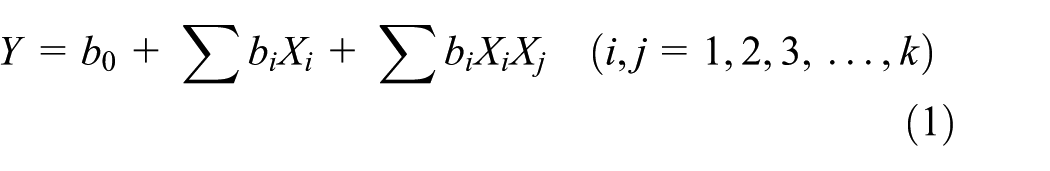
where

With Y being the predicted response,

where
Welding parameters used in this study.
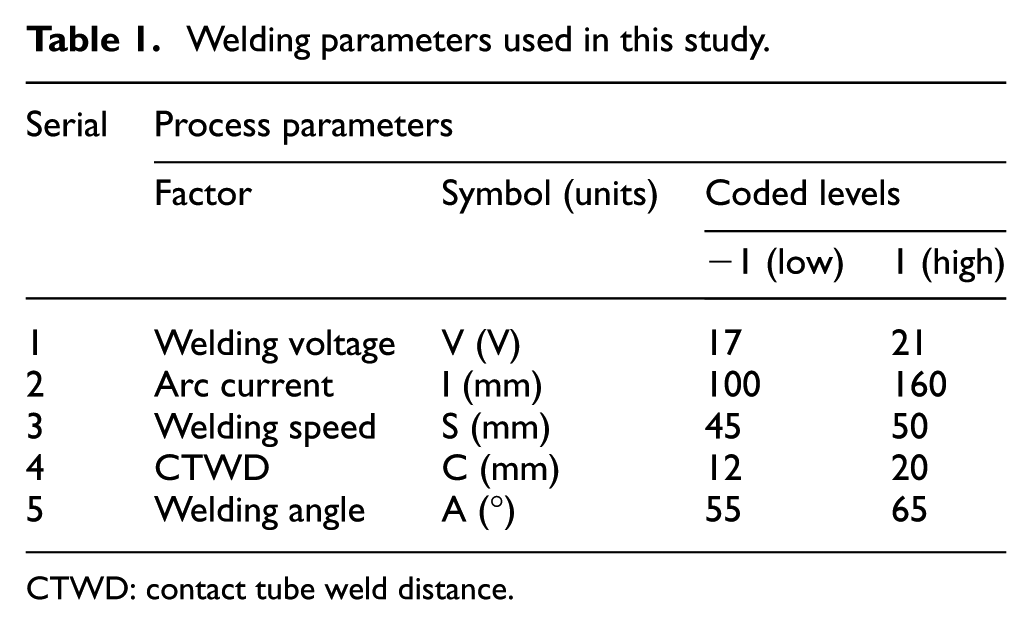
CTWD: contact tube weld distance.
Results and discussion
RSM model
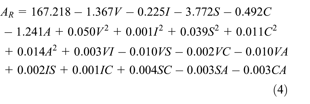
Experiments were performed following the design matrix shown in Table 2. Model coefficients from equation (2) were estimated using multiple regression analysis
Analysis of variance for the response surface method model for bead reinforcement area.

Figure 3 compares measured and predicted bead reinforcement area. The prediction model shows good agreement with the experimental results.
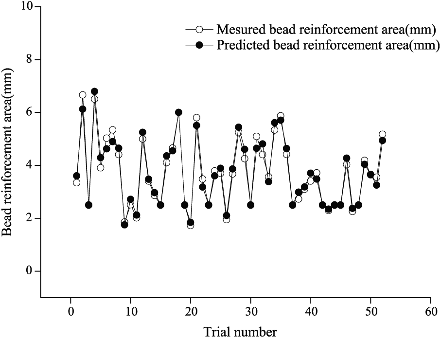
Measured and predicted bead reinforcement area.
The mathematical relationships employed for estimation of the analysis of variance (ANOVA) estimators were usually used in the literature regarding design of experiment (DOE) and RSM. The coefficient of determination (R2) was employed to investigate fit quality for the various models (linear, two factor, and quadratic). R2 explains the total deviation about the mean,23,24 with larger R2 (close to unity) implying a better model that provides predicted response values close to the actual values. Thus, R2 = 0.893 indicates good agreement between observed and predicted bead reinforcement area.
The model was also assessed for suitability using an ANOVA, as shown in Table 2. The quadratic model lack of fit is significant (p = 0.198), which confirms the relatively low R2 = 0.893 for the overall model.
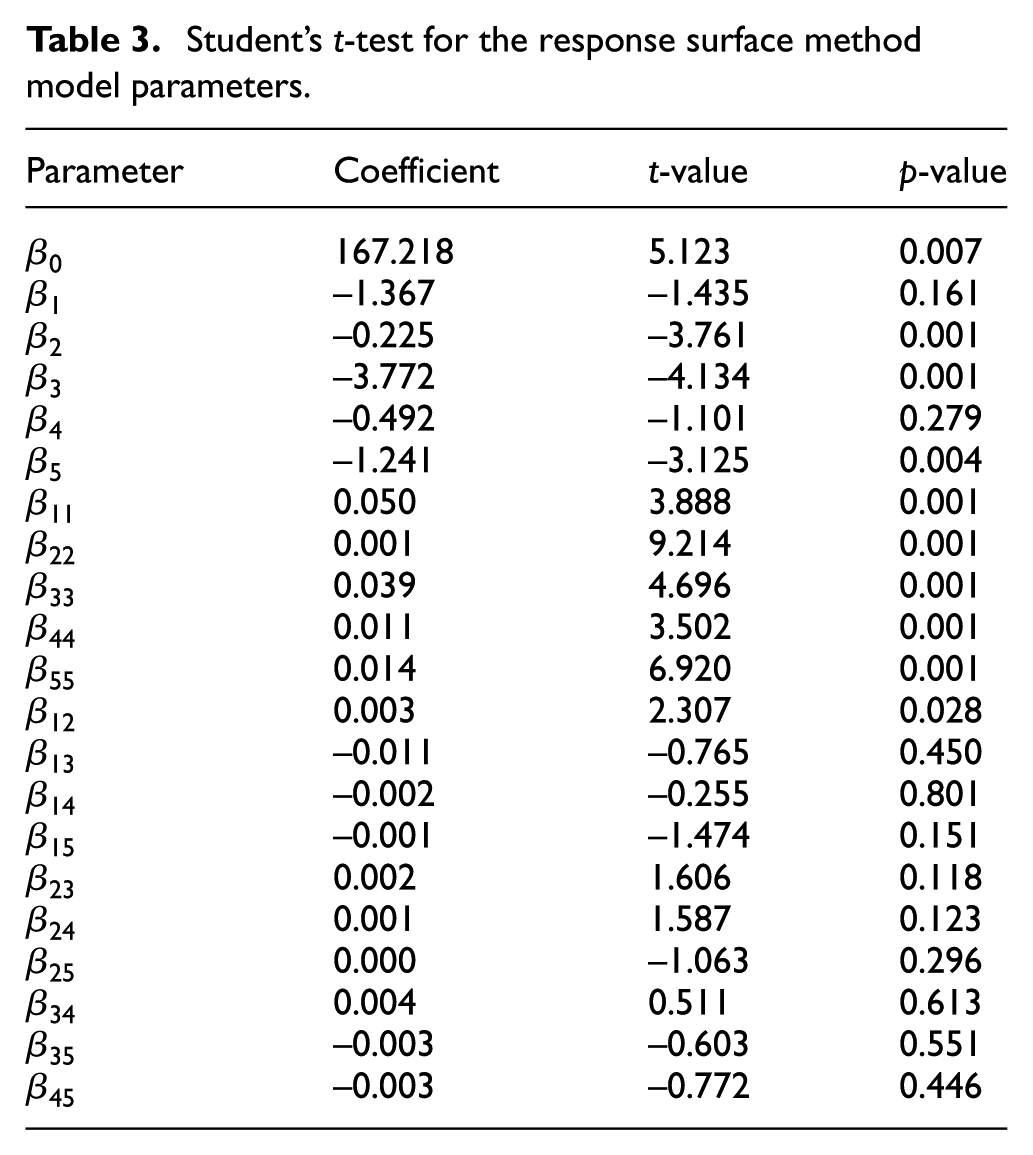
Table 3 shows Student’s t-test for the RSM model parameter terms. The p-value indicates the relative importance of each parameter at a specified level of significance, with higher t-value or smaller p-value implying more significance.
17
Generally, p-value < 0.05 (significant at the 95% level or better) is considered to be very significant and contributes largely toward the response. Squared terms have the largest effect on bead reinforcement area with p < 0.001, that is, 99.9% confidence, and the highest absolute t = 9.214. Other significant terms (exceeding 95%) include
Student’s t-test for the response surface method model parameters.
ANN model
The ANN predictive model was based on the Levenberg–Marquardt BP (LMBP) neural network algorithm to train the multi-layer perceptron (MLP) network, which has better learning rate and relative stability compared to the original BP algorithm. 21 The Levenberg–Marquardt (LM) algorithm is an approximation of a Gauss–Newton algorithm, which enables much quicker learning than the BP algorithm, which is based on a steepest descent algorithm. The LM modification to the Gauss–Newton algorithm is calculated as
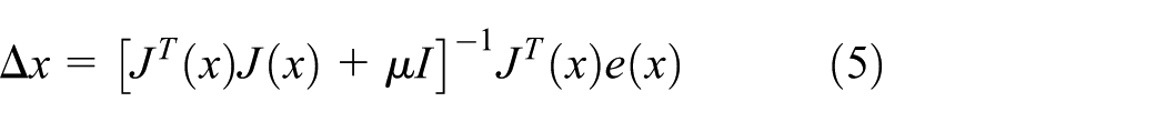
where μ is the Marquardt adjustment parameter and I is an identity matrix. When μ is small, the LM algorithm approximates the Gauss–Newton algorithm.25,26
MATLAB was employed to develop the network and its training, and various neural network functions were employed for the wide ranging input variable compositions to predict the complicated and nonlinear output variables. Physical data were measured three times with the average used for training. To select the ANN structure, six different neural network configurations were evaluated, as shown in Table 4. The number of neurons on the hidden layer was fixed at three.
Characteristics of the six selected ANNs.

ANN: artificial neural network; MSE: mean square error.
The transfer function (also called the system or network function) is a mathematical representation of the relationship between the input and output in terms of spatial or temporal frequency. Transfer functions usually have a sigmoid shape, but they may also have other nonlinear forms, such as piecewise linear or step functions. They are usually monotonically increasing, continuous, differentiable, and bounded.
One of the most common transfer functions is Log-sigmoid (Logsig), as shown in Figure 4(a), which is differentiable and maps any input value between plus and minus infinity to [0,1]. The hyperbolic tangent transfer function, as shown Figure 4(b), is a bipolar sigmoid with output [−1,+1]. It is similar to tanh (n), although it can be calculated somewhat quicker. This function is a good trade-off for neural networks, where speed is more important than the exact shape. Most real models have nonlinear input/output parameters, but some models are close to linear within nominal parameters, that is, not over driven. Thus, a linear transfer function (Purelin) as shown Figure 4(c) can be an acceptable representation of the input/output behavior for these situations. 27

ANN transfer functions considered: (a) Log-sigmoid:
ANN configurations 1 (logsig + logsig as transfer functions), 2 (tansig + purelin as transfer functions), and 6 (tansig + purelin) use the trainlm training function. Trainlm is based on the LM algorithm and locates the minimum of a multivariate function that can be expressed as the sum of squares of nonlinear real-valued functions. This is an iterative technique such that the performance function will always reduce in each iteration. Thus, trainlm is the fastest training algorithm for networks of moderate size. However, trainlm has the drawback of memory and computation overhead due to calculating the gradient and approximated Hessian matrix. 28
ANN configurations 3 (logsig + logsig as transfer functions), 4 (tansig + purelin as transfer functions), and 5 (tansig + purelin as transfer functions) use the trainbr training function, which updates weights and biases according to LM optimization, minimizing a combination of squared errors and weights, and determining the correct combination to produce a network that generalizes well.29,30
ANN 5 is the same as ANN 4, aside from µ = 0.01 and 0.005, respectively. Similarly, ANN 6 and ANN 2 use µ = 0.01 and 0.005, respectively.
Figure 5 shows the fit quality (R2) for considered ANN configurations. Transfer function tansig + purelin provided better results than logsig + logsig. However, Figure 5(a) and (c) and Table 6 show that R2 and mean square error (MSE) increased for the test sets compared with the training sets using logsig + logsig, that is, the neural network did not work well, resulting in a large dispersion. However, tansig + purelin shows decreased MSE and increased R2 for the test sets (Table 4 and Figure 5(b), (d), (e), and (f)). For constant

Model fits for the selected artificial neural network (ANN) bead reinforcement area models: (a) ANN 1, R2 = 0.859; (b) ANN 2, R2 = 0.943; (c) ANN 3, R2 = 0.834; (d) ANN 4, R2 = 0.923; (e) ANN 5, R2 = 0.948; and (f) ANN 6, R2 = 0.915.
Comparison of RSM and ANN models
Eight additional experiments, as shown in Table 5, were performed to select the most accurate model for prediction of bead reinforcement area, with RSM and ANN outcomes shown in Figure 6. Generally, ANN has superior performance than RSM.
Bead reinforcement area model parameters for model comparison.

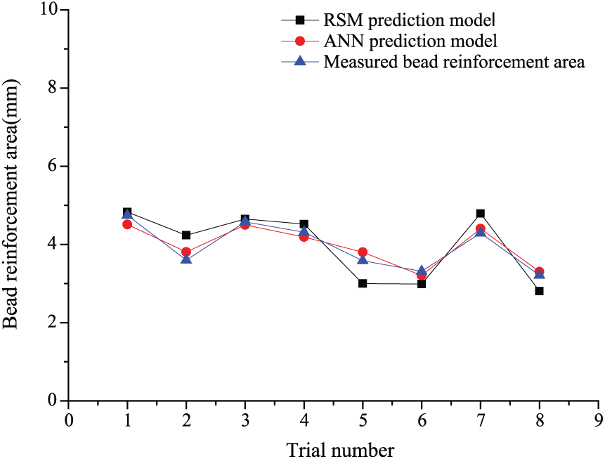
Bead reinforcement area (AR) prediction by response surface method (RSM) and artificial neural network (ANN) models.
The response of predicted

where
Prediction model performance.

RSM: response surface methodology; ANN: artificial neural network; AAD: average absolute deviation.
Conclusion
This article studies the performance of RSM- and ANN-based models to estimate bead reinforcement area in GMA welding. Both models provide good quality predictions using five welding parameters (voltage, arc current, welding speed, CTWD, and welding angle), but ANN prediction was significantly superior to RSM (R2 = 0.893 and 0.948, ADD = 4.01% and 3.11% for RSM and ANN, respectively) for both data fitting and estimation. Therefore, a rule-based expert system could be based on the ANN prediction model to provide optimized automatic GMA welding. This would allow simple bead reinforcement area prediction and confident deployment of automated GMA systems.
Footnotes
Handling Editor: Yaguo Lei
Declaration of conflicting interests
The author(s) declared no potential conflicts of interest with respect to the research, authorship, and/or publication of this article.
Funding
The author(s) received no financial support for the research, authorship, and/or publication of this article.