Sage Journals: Discover world-class research

Abstract

To study the significance of internal pressure pulsation characteristics between prototype and model pump devices, monitoring of computational fluid dynamics and dynamic measurement of a model were carried out under different working conditions and measuring points. The results of computational fluid dynamics calculation and model test are as follows. First, the positions of main frequency and subfrequency are almost the same, whereas the amplitude has a slight deviation. Second, the amplitude of inlet impeller is larger, and the main frequency is three times of rotating frequency. Third, the inlet speaker has mainly low pulsation, which is almost distributed in blade frequency and 1/3 times of rotating frequency. Moreover, the pressure pulsation of symmetrical points in each condition has a good symmetry. As the flow rate decreases, both the mixing and blade frequency amplitudes in the inlet speaker and impeller first decrease and then increase. The minimum mixing amplitude appears in the design condition of 253 L/s, whereas the blade frequencies are 203 and 253 L/s. The numerical calculation results are almost the same as those of prototype and model devices. Therefore, numerical calculations and experimental studies on pressure pulsation can guide the design and stable operation of similar pump stations.

Keywords

Prototype and model pump devices pressure pulsation numerical calculation test analysis

Introduction

Axial-flow pumps are widely used because of the advantages of a small engineering investment, a simple structure, easy installation and maintenance, and stable operation.^1–3

In recent years, with more and more applications of axial-flow pumps,⁴ much attention has been paid to its efficiency, safety, and stability. Pressure pulsation is a key parameter reflecting the stability. The internal pressure pulsation of prototype and model axial-flow pumps has been rarely studied. Moreover, a combination of numerical calculations and model tests has not been widely used to investigate the internal pressure pulsation of axial-flow pumps.^5–9 Most of the studies focused on centrifugal pump,^10,11 mixed flow pump,¹² and hydraulic turbine.¹³

In this study, the internal pressure pulsation of prototype and model axial-flow pumps was investigated. The relationship between the internal pressure pulsation of an axial-flow pump and that obtained from the numerical calculation of prototype and model devices under different working conditions and measurement points was established. The pressure pulsation accuracy of the axial-flow pump was verified by performing a model test. These studies provide a reference for the prediction, test, and theoretical analysis of pressure pulsation for other pump stations.

Overview of pump station project

A new water control pump station used a vertical axial-flow pump equipped with an X-type two-way flow channel and fully adjustable blades. The flow of prototype single pump was 33.4 m³/s, and the flow of the total installation was 300 m³/s. The main parameters—impeller diameter, speed, flow, and head (including gate slot loss)—of the prototype and model pumps are shown in Table 1.

Table 1.

Main parameters of pump station.

Pump device	Impeller diameter	Speed	Flow	Head
Pump device	mm	rpm	L/s	m
Model device	300	1150	253	1.36
Prototype device	3450	100	33,459	1.36

Numerical calculation

Calculation model

An axial-flow model pump uses a box-type inlet and outlet flow channel. In this article, the Design Model (DM) module of ANSYS¹⁴ software was used for the parametric modeling of inlet and outlet channels based on the flow-path size of prototype and model pumps. Figure 1 shows the calculation model for the box-type axial-flow pump.

Figure 1.

Numerical model of box-type inlet runner.

Water first flows through the inlet channel and then driven by the impeller. Directed by the guide vane, the water then enters the outlet channel and finally flows out.

Meshing

The built model can be meshed using the ANSYS ICEM software. Using this method, Figures 2 and 3 show the generated hexahedral-structured grid of box-type inlet and outlet channel, respectively, leading to the boundary layer and local encryption. The grid number and grid nodes are shown in Table 2. In addition, the grid quality is more than 0.37.

Figure 2.

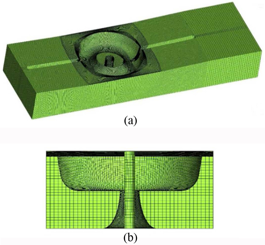
(a) Box-type inlet channel: overall structured grid and (b) box-type inlet channel: partially structured grid.

Figure 3.

(a) Box-type outlet channel: structured grid and (b) box-type outlet channel: structured grid.

Table 2.

Grid node and grid number.

Vertical axial-flow pump
Calculation domain	Node number	Grid number
Impeller domain	820,566	778,722
Guide vane domain	518,765	480,150
Outlet channel	1,100,166	1,057,464
Inlet channel	649,446	616,308
Total	3,088,943	2,932,644

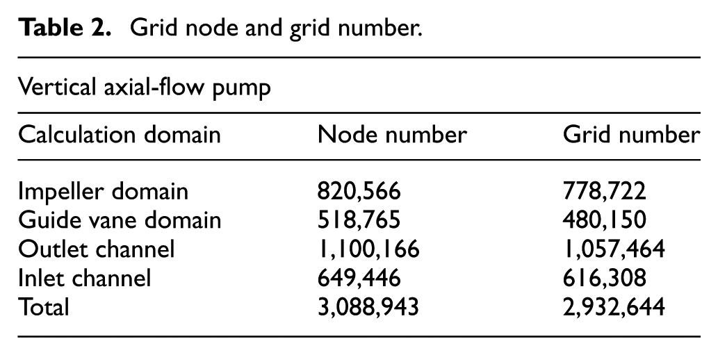
For numerical calculation, the number of blades in the hydraulic model of axial-flow pump is three, and the number of vanes is five. The solid modeling and meshing of impeller and guide vane were carried out using the ANSYS TurboGrid software. Figure 4(a) shows the model of impeller and guide vane. Figures 4(b)–(e) show the structured grids of impeller and guide vane. The grid number is shown in Table 2. Based on a standard model pump, D is equal to 300 mm during the modeling, and the unilateral blade clearance is 0.2 mm.

Figure 4.

Impeller, vane model, and grid: (a) model of axial-flow pump impeller and guide vane, (b) impeller grid: vertical figure, (c) impeller grid: front figure, (d) guide vane vertical grid, and (e) guide vane front grid.

The requirements of grid independence are reported in Yang and Liu.¹⁵ In this study, by changing the grid number of overall pump and calculating its efficiency, it was found that when the grid number increases to a certain number, the efficiency no longer increases and remains stable, as shown in Figure 5. To satisfy the requirements of grid independence, when the grid number of impeller was 778,722, the grid number of vane was 480,150 and the grid number of entire pump was 2,932,644. The calculation results show that when the y+ value is about 35, the requirements are satisfied.

Figure 5.

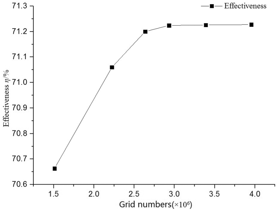
Verification of grid independence and performance prediction.

Constant boundary conditions and control equations

The grid model of each segment was imported into CFX-Pre, and a pump model was built. Using the Computational Fluid Dynamics (CFD) calculation method, the speeds of model and prototype pumps were set to 1150 and 100 rpm, respectively, and the parameters (flow, head, and efficiency) are shown in Table 3. The total outlet pressure of prototype and model pumps was set to 1 atm. The inlet channel, outlet channel, impeller shell, and guide vane of axial-flow pump were set as the stationary wall, and nonslip conditions were applied. The near-wall region used the boundary condition of standard wall function.

Table 3.

Results predicted from prototype and model pumps.

Pump device	Flow	Head	Efficiency
Pump device	Q (L/s)	H (m)	η (%)
Prototype	16,663.5	3.94029	55.7592
	20,102	3.43002	62.4609
	26,846.75	2.49616	70.814
	33,459.25	1.6153	75.5262
	37,691.25	0.711722	55.3655
Model	126	3.90417	54.6339
	152	3.39767	61.2154
	203	2.40101	67.9929
	253	1.5174	71.2242
	285	0.593768	47.0353

The relative position of rotating impeller and guide vane does not affect the dynamic and static interface. A “Stage” interface was used to control the transmission of parameters between the impeller and guide vane. The discretization of control equation was based on the finite-volume method. The diffusion term and pressure gradient were represented by finite-element function. The convective term uses a high-resolution scheme. The inside of pump uses the Reynolds-averaged Navier–Stokes (N-S) equation. Considering the rotation in the average flow, the turbulence model uses the renormalized group (RNG) k–ε turbulence model. These can better handle a high strain rate and flowline bending of a large flow.

In the preprocessor, first the pressure increments and efficiency expression of pump inlet and outlet cross-sections were written. Then, as an auxiliary monitoring point, a real-time observation was considered during the calculation. The convergence condition was the residual value of 10e – 5, and the pressure increment and efficiency of pump’s inlet and outlet section were monitored till they were stable.

Calculation formula

Prediction of energy performance of pump

The pump head was calculated using the Bernoulli energy equation, and the obtained velocity field, pressure field, and torque acting on the impeller were used to predict the hydraulic performance. The total energy difference between the inlet and outlet of the pump is defined as unit head. Device head is defined as the total energy difference between the inlet and outlet flow channel, as shown below

\begin{array}{l} H_{n e t} = (\frac{\int_{S_{2}} p_{2} u_{t 2} d S}{ρ Q g} + H_{2} + \frac{\int_{S_{2}} {u_{2}}^{2} u_{t 2} d S}{2 Q g}) \\ - (\frac{\int_{S_{1}} p_{1} u_{t 1} d S}{ρ Q g} + H_{1} + \frac{\int_{S_{1}} {u_{1}}^{2} u_{t 1} d S}{2 Q g}) \end{array}

(1)

H ₁ and H₂ are the inlet and outlet section elevations of pump, unit: m; S₁ and S₂ are the inlet and outlet section areas of pump, unit: m²; u₁ and u₂ are the inlet and outlet flow rates of pump, unit: m/s; u_t₁ and u_t₂ are the inlet and outlet flow rates of a normal component of pump, unit: m/s; and the efficiency of pump can be calculated as follows

η = \frac{ρ g Q H_{n e t}}{T_{p} ω} \times 100 %

(2)

T_p is the torque, unit: N·m; and ω is the rotational angular velocity of impeller, unit: rad/s.

Unsteady calculation settings and monitoring point location

Unsteady calculation settings

In this study, the impeller rotation for the unsteady calculation of time step of prototype and model pumps is about 1/120 of a cycle. The impeller rotates only 3° at each time step. On one hand, for a model pump, the total time is 0.313 s. This is also the time taken by the impeller to rotate six cycles. Therefore, it can be concluded that the time taken for each step is 0.000434 s. On the other hand, for a prototype pump, the total time is 3.6 s. Using the same calculation method, the time taken for each step is 0.005 s. In the calculation, first the impeller was fixed at a certain position to calculate the three-dimensional steady turbulence. Second, the steady flowfield result was used as the initial flowfield calculated from the unsteady turbulence. Third, the convergence condition was set to the residual value of 10e – 6.

Unsteady calculation of monitoring point location

To monitor the pressure pulsation in each position of axial-flow pump, two monitoring points were arranged on the back wall of inlet horn and impeller. The prototype pump is about 11.5 times the size of model pump. According to this conversion, the coordinate data of prototype pump monitoring point can be obtained. The locations of monitoring points of prototype and model pumps are shown in Figure 6.

Figure 6.

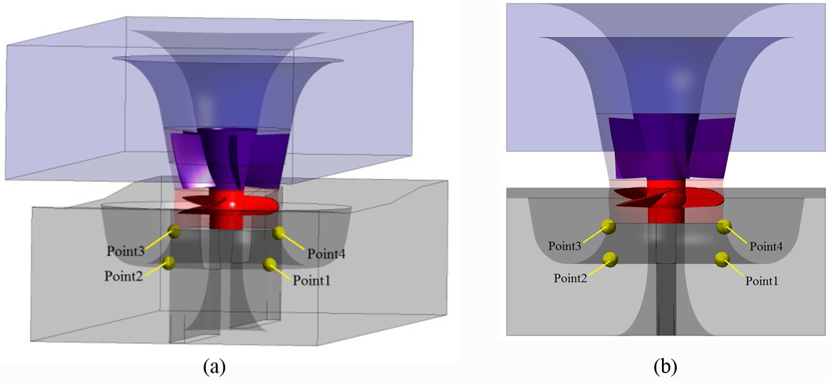
(a) Monitoring points for pressure pulsation: overall figure and (b) monitoring points for pressure pulsation: front figure.

Steady numerical calculation results of prototype and model pumps

When the blade placement angle of prototype and model pumps is −3°, the steady numerical calculation of five characteristic flow points was carried out. The results are shown in Table 3.

In addition, a comparison of the hydraulic characteristics of prototype and model pumps is shown in Figure 7. In the comparison, the flow rate and vanishing method are dimensionless. The dimensionless formulas are as follows

K_{Q} = \frac{Q}{n D^{3}}

(3)

K_{H} = \frac{H}{n^{2} D^{2}}

(4)

Figure 7.

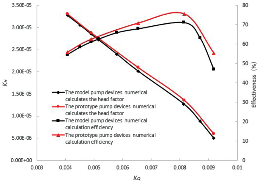
Comparison of numerical simulation performance of prototype and model pumps.

The efficiency of design point can be increased to 4% from the contrast curve of prototype and model pumps. This indicates that when the design condition of the pump is 253 L/s, the pump operation is good. Compared with a small increase at a slight flow rate of prototype pump, at a large flow rate, the efficiency of pump reached the maximum, up to 8%. This shows that when the model pump was extended to the prototype pump, the local hydraulic loss inside the pump unit is reduced. However, it also has a relationship with the flow. When the flow rate is large, the local hydraulic loss has a significant reduction. Moreover, the efficiency of pump significantly increases.

Comparison of unsteady numerical results of prototype and model pumps

This study shows that the pressure pulsation waves in the last three of the six cycles of pump remain stable. First, it is necessary to obtain the data of each static pressure monitoring point in the last three cycles. Then, through the fast Fourier transform, in the design condition Q_s, the comparison curve of the pressure fluctuation spectrum of prototype and model pump’s monitoring points was obtained as shown in Figures 8 –11. The pressure pulsation spectrum of prototype pump can be calculated in terms of the multiple of prototype pump frequency (f_p = 100/60). Moreover, the pressure pulsation spectrum of model pump can be calculated in terms of the multiple of model pump frequency (f_m = 1150/60).

Figure 8.

Point 1 comparison chart of pressure pulsation from measuring point 1.0 Qs by prototype and model numerical calculation.

Figure 9.

Point 2 comparison chart of pressure pulsation from measuring point 1.0 Qs by prototype and model numerical calculation.

Figure 10.

Point 3 comparison chart of pressure pulsation from measuring point 1.0 Qs by prototype and model numerical calculation.

Figure 11.

Point 4 comparison chart of pressure pulsation from measuring point 1.0 Qs by prototype and model numerical calculation.

The pressure pulsation results of prototype and model pump’s design conditions show that the results of prototype pump are similar to those of model pump. Furthermore, based on similar measuring points of prototype and model pumps, the amplitude and magnitude of pressure pulsation are similar.

Model test device

The pressure pulsation test of a box-type model pump was performed. The measuring points are located in the position of speaker tube and impeller inlet. The two points are shown in Figure 12. In addition, the pressure pulsation measuring point and coordinates of box-type pump are shown in Table 4.

Figure 12.

Sensor measuring point layout.

Table 4.

Measuring points and coordinates of model pump.

Position of measuring points	X (m)	Y (m)	Z (m)	Remark
Point 1	−0.145	−0.145	−0.155	Northeast of inlet speaker
Point 2	−0.145	0.145	−0.155	Southeast of inlet speaker
Point 3	0	0.15	−0.07	South of inlet impeller
Point 4	0	−0.15	−0.07	North of inlet impeller

A high-frequency dynamic micro CYG505 sensor was used, and the outer diameter was 5 mm. The characteristics were small size, small flowfield disturbance, high sensitivity, and good dynamic frequency response. The range was from −100 to 100 kPa. The sampling frequency was 100 kHz. The output was from 0 to 5 V, and the accuracy level was 0.25%. This sensor was also waterproof. The acquisition instrument was SQQCP-USB-16. The sensor was installed perpendicular to the wall. The test system and acquisition device are shown in Figure 13.

Figure 13.

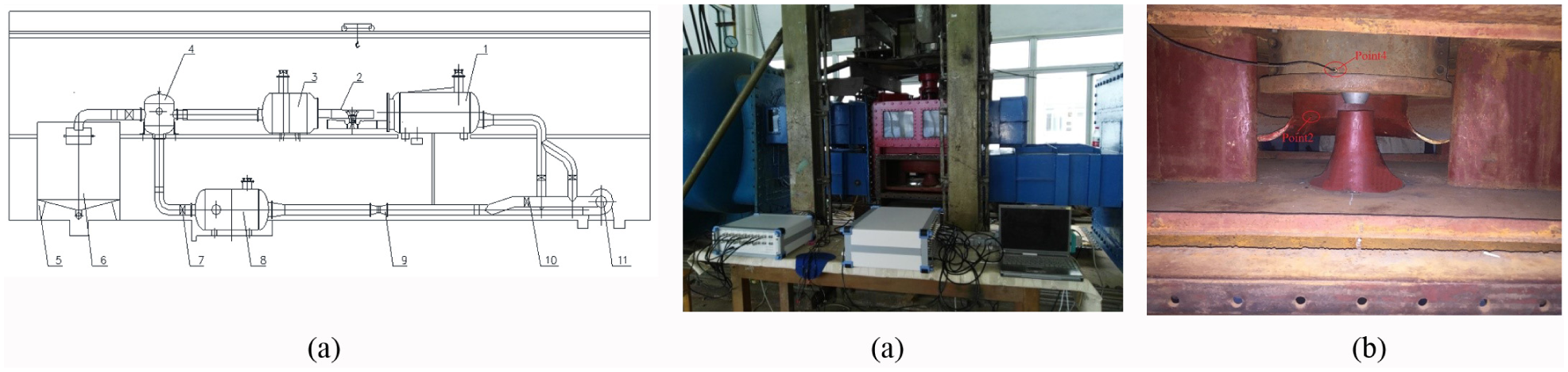
Physical map of pump pressure pulsation test: (a) high-precision hydraulic machinery test system, (b) pulsation test: acquisition device, and (c) pulsation test: sensor.

The following tests were carried out for the model pump:

Energy performance test of model pump under leaf angle,

−3° pressure pulsation test for five flow points under blade placement,¹⁶

Test implementation of the “centrifugal pump, mixed flow pump, and axial-flow pump hydraulic performance test specifications (precision level)” (GB/T 18149-2000) and “pump model and device model acceptance test procedures” (SL140-2006) standards. With more than 18 performance testpoints of each blade placement angle, the pressure pulsation test became stable.

Contrastive analysis of numerical results and model test

Contrastive analysis of steady results of numerical calculation and external characteristics of the test

Figure 14 shows the results of model test. When the blade placement angle of model pump was −3°, steady numerical calculation of characteristic flow points was performed. Moreover, the head and efficiency were also calculated. A comparison between the numerical calculation and external characteristics of the test is shown in Figure 15.

Figure 14.

Complete characteristic curve of pump’s model test.

Figure 15.

Contrastive analysis curve of external characteristics of numerical calculation and model test.

The model test results of pump show that when the flow was 253 L/s, the pump head was 1.36 m and the efficiency was 65%. Thus, the design of the pump is more accurate, impeller selection is reasonable, and efficient operation range is wide. The maximum operating head of the pump was >3.45 m, satisfying the maximum operating water level. In addition, the critical runoff margin was designed to the smallest, at about 3.5 m, satisfying the requirements of critical ablation margin of pump station.

Compared with the test, some deviations were observed in the prediction of steady numerical calculation. However, the deviation is less than 3%, satisfying the requirements of engineering and scientific research. Some deviations were also observed in the prediction of large and small flow conditions. This is mainly because the internal return flow range is large, leading to very small hydraulic loss prediction under large flow conditions, very large loss prediction under small flow conditions, and more accurate design point.

Contrastive analysis of numerical calculation and pressure fluctuation test

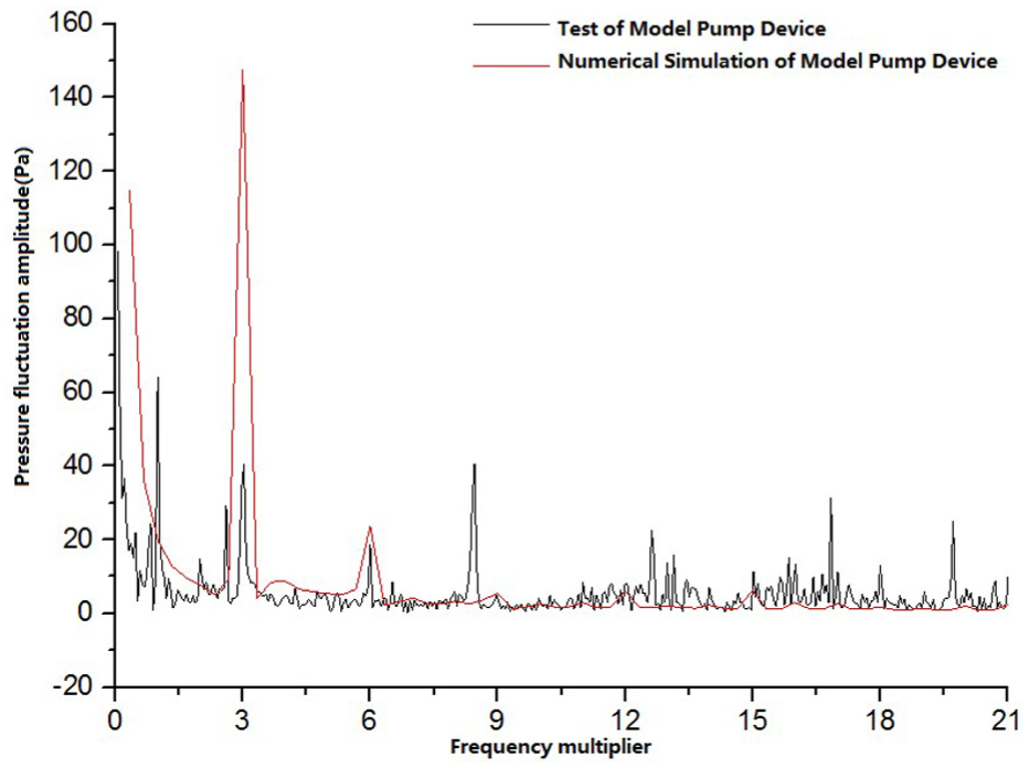
When the blade placement angle of model pump was −3°, through the numerical calculation of characteristic flow point, the contrastive frequency domain charts of pressure pulsation and model test are shown in Figures 16 –19. The numerical calculation of model pump and pressure pulsation test were carried out in multiples of model pump rotating frequency (f_m = 1150/60).

Figure 16.

Contrastive frequency domain chart of numerical calculation and pressure pulsation test when testpoint 1 is at Qs = 253 L/s.

Figure 17.

Contrastive frequency domain chart of numerical calculation and pressure pulsation test when testpoint 2 is at Qs = 253 L/s.

Figure 18.

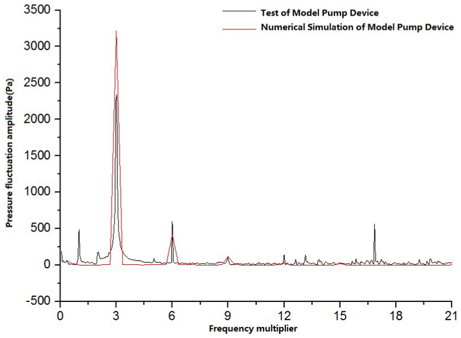
Contrastive frequency domain chart of numerical calculation and pressure pulsation test when testpoint 3 is at Qs = 253 L/s.

Figure 19.

Contrastive frequency domain chart of numerical calculation and pressure pulsation test when testpoint 4 is at Qs = 253 L/s.

According to the analysis chart of numerical calculation and pressure pulsation test from points 1 and 2 in the inlet flow of model pump, the following conclusions can be drawn. First, the predicted value of model pump is larger than the value of pressure pulsation test. Second, the main frequency position is reasonable. Third, the amplitude prediction has a slight deviation. Finally, the deviation of high-frequency part is slightly larger.

According to the analysis of numerical calculation prediction and pressure pulsation test from points 3 and 4 in the inlet impeller of model pump as shown in Figures 18 and 19, the following conclusions can be drawn. The numerical calculation results are almost consistent with the prediction of inlet impeller amplitude and pressure pulsation results of model test, and the deviation is very small. The numerical calculation results can also be used instead of a model test to determine pressure pulsation. The value obtained, which is very conservative, completely satisfies the pump’s safe and stable operation requirements.

Relationship between the mixing frequency amplitude of pressure pulsation and working condition, testpoint

The inlet water part includes four testpoints for pressure pulsation. They are located in the south, north of inlet impeller, and the northeast and southeast of inlet speaker tube. During the test of model pump’s pressure pulsation, 126, 152, 203, 253, and 285 L/s were taken as the flow points. The mixing amplitude of pressure fluctuation is the sum of amplitudes at each frequency after the fast Fourier transform. The relationship between the mixing amplitude and flow rate of pressure pulsation at all the testpoints is shown in Figures 20 and 21.

Figure 20.

Flow changes versus the mixing frequency chart of pressure pulsation at each testpoints in the inlet water speaker.

Figure 21.

Relationship between the pressure pulsation mixing amplitude and change in flow rate at the testpoint of inlet impeller.

The numerical calculation results and pressure pulsation test of model pump shown in Figure 20 indicate that as the flow decreases, the pressure pulsation first decreases and then increases. In the design case 253 L/s, the amplitude of pressure pulsation is the smallest. When the flow rate is large and small, the amplitude of pressure pulsation clearly increases. Near the design case, the amplitude clearly does not change.

The numerical calculation results and pressure pulsation test of model pump show that the amplitudes of testpoints 1 and 2 in the inlet water speaker are very symmetrical. Moreover, the amplitude is consistent with the trend of flow. However, a numerical difference was observed, mainly because the minimum frequency of numerical simulation and pressure pulsation test is not the same. The minimum frequency is related to the sampling frequency of numerical calculation and pressure pulsation test. The smallest sampling period of the test was 0.000001 s. The numerical simulation was limited by the calculation resource, and the sampling period was 0.00004348 s. It is difficult to perform numerical simulations of a sample at the same time interval as the pressure pulsation test of model pump. Therefore, the degree of test separation is greater, and the stack will provide different values. The analysis of trend shows that the results are more consistent.

The results of numerical simulation and pressure pulsation test of model pump shown in Figure 21 indicate that the design condition at this testpoint is the best. The amplitude of pressure fluctuation under a large flow condition does not clearly increase. Its magnitude is larger, the slope of the curve significantly changes, and the flow slightly changes. The variation in mixing amplitude is significantly different from that in the inlet and outlet flow channels. When running to a small flow area, the slope of pressure pulsation amplitude is larger and the growth rate is rapid. Therefore, it is necessary to avoid running under a small flow condition.

The numerical calculation results and pressure pulsation test of model pump show that the amplitudes of testpoints 3 and 4 in the inlet impeller are very symmetrical. Moreover, the amplitude is consistent with the flow trend. However, a numerical difference was observed, mainly because the sampling frequencies of numerical simulation and pressure pulsation test are not the same. The specific reasons were explained earlier in this article.

Relationship between pressure pulsation of blade frequency, amplitude, and working condition, testpoint

After the previous analysis, the pressure pulsations at 3, 6, 9, 12, and 15 times were summed to obtain the pressure pulsation amplitude associated with the blade frequency. The relationship between the pressure pulsation and flow rate of measured blade is shown in Figures 22 and 23.

Figure 22.

With the change in flow, the frequency chart of pressure pulsation at each testpoint in the inlet water speaker.

Figure 23.

Flow changes versus the frequency chart of pressure pulsation at each testpoint in the inlet impeller.

The results of numerical calculation and pressure pulsation test of model pump shown in Figure 22 indicate that as the flow changes, the pressure pulsation of blade frequency clearly changes. When the flow decreases, the pressure pulsation first decreases and then increases. In the design case 203 L/s, the amplitude of pressure pulsation is the smallest. When the flow rate is large and small, the amplitude of blade frequency clearly increases. The results of numerical calculation and pressure pulsation test of model pump show that these two testpoints are very symmetrical.

The results of numerical simulation and pressure pulsation test of model pump show that the change in frequency amplitude of inlet speaker and blade is consistent. The amplitude is similar, and the deviation is small, indicating that numerical simulation can be used instead of model test pressure pulsation.

The results of numerical calculation and pressure pulsation test of model pump shown in Figure 23 indicate that at testpoints 3 and 4, as the flow decreases, the pressure pulsation of impeller frequency increases. When the flow is >203 L/s, the amplitude of inlet impeller is smaller and the change is not clear. When the flow is <203 L/s, the amplitude clearly increases. The results of numerical calculation and pressure pulsation test of model pump indicate that these two testpoints are very symmetrical.

The results of numerical simulation and pressure pulsation test of model pump show that the change in frequency amplitude of inlet impeller is consistent. The amplitude is similar, and the deviation is small, indicating that the prediction of numerical simulation is accurate.

Flow regime analysis of box-type axial-flow pump under different working conditions

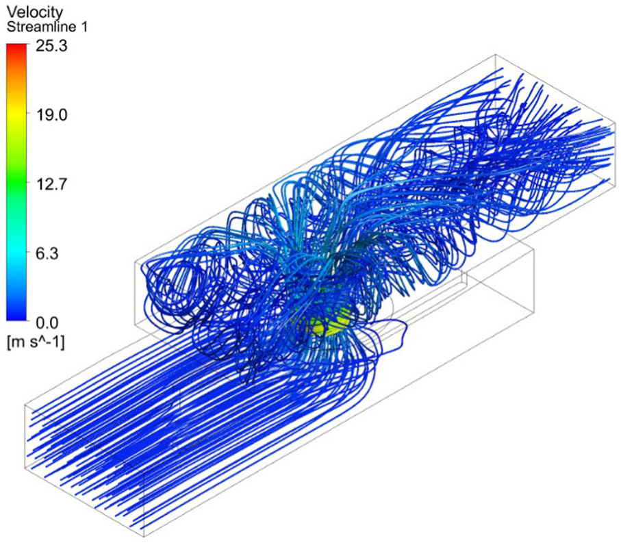
The flowlines of overall model device under the working conditions of 285, 253, 203, 152, and 126 L/s were removed as shown in Figures 24 –28.

Figure 24.

Streamline of model device under the working condition of Q = 285 L/s.

Figure 25.

Streamline of model device under the working condition of Q = 253 L/s.

Figure 26.

Streamline of model device under the working condition of Q = 203 L/s.

Figure 27.

Streamline of model device under the working condition of Q = 152 L/s.

Figure 28.

Streamline of model device under the working condition of Q = 126 L/s.

The flowline figure of the overall pump device shows that from a large flow condition of 285 L/s to a small flow condition of 126 L/s, the flow regime of box-type device first became better and then became worse. This trend is the same as pressure pulsation. This is mainly because a box-type device with four gates was used to achieve bidirectional operation. However, a dead water zone in the blind end of inlet channel cannot be avoided, and the flow regime is very poor. Therefore, it is important to study this phenomenon that can effectively avoid safety accidents and guide the design of box-type axial-flow pumps.

Conclusion

By comparing the results of a test and steady prediction of a model pump, the deviation was found to be within 3%. This satisfies the needs of engineering and research. The results of a nondimensional comparative analysis of prototype and model pumps indicate that due to the scale effect, the efficiency of prototype pump is higher than that of model pump.

The results of a contrast analysis of numerical calculation using prototype and model pumps indicate that in units of rotating frequency, the spectral components of pressure pulsation are similar and the amplitude is equivalent. The numerical predictions of prototype and model pumps are similar.

The numerical prediction and test of model pump at all the 1, 3, 6, 9, 12, and 15 times the rotating frequency show that the pump has a pressure pulsation peak. The pressure pulsations of numerical calculation prediction and test are at the same frequency, and the amplitude is larger. This indicates that numerical calculation can be used to predict the pressure pulsation that is reliable. Numerical calculation can generally achieve the hydraulic pulsation of a model pump with a certain margin of safety.

The results of numerical calculation and pressure pulsation test of a model pump show that both the testpoints of inlet speaker and impeller chamber are symmetrical. As the flow changes, the amplitude of numerical simulation and pressure pulsation test of model pump are consistent. When the design conditions are optimal, both large and small flow conditions increase.

The results of numerical simulation and pressure pulsation test of model pump show that the change in frequency amplitude of blade is consistent. The amplitude is similar and the deviation is small. When the design conditions are optimal, both large and small flow conditions increase. This indicates that numerical simulation prediction can be used instead of model test pressure pulsation.

The results of analysis of internal pressure pulsation characteristics calculated by numerical simulation and model test show that a high-frequency alignment is not so high as a low-frequency alignment. This indicates that improvement is necessary during the numerical simulation and model test. Moreover, based on this study, pressure pulsation points should be increased, revealing the time and space distribution characteristics of a box-type pump. It also provides a systematic research, induction, and further elucidation of its mechanism.

Footnotes

Handling editor: Hyung Hee Cho

Declaration of conflicting interests

The author(s) declared no potential conflicts of interest with respect to the research, authorship, and/or publication of this article.

Funding

The author(s) disclosed receipt of the following financial support for the research, authorship, and/or publication of this article: This research work was supported by the National Natural Science Foundation of China (Grant nos. 51376155 and 51609210); China Postdoctoral Science Foundation–funded projects (2016M591932); A project funded by the Priority Academic Program Development (PAPD) of Jiangsu Higher Education Institutions and Jiangsu Province scientific research and innovation project (KYZZ16_0492). Support for construction/assembly of the facility was also provided by the Hydrodynamic Engineering Laboratory of Jiangsu Province.

ORCID iD

Chuanliu Xie

References

Liu

. Water pump and pump station. Beijing, China: China Water Conservancy and Hydropower Press, 2009.

Shi

Zhang

Jin

et al . A study on tip leakage vortex dynamics and cavitation in axial-flow pump. Fluid Dyn Res 2001; 49: 035504.

Wang

. An analysis on the flow characteristics of bi-directional axial-flow pump under reverse operation. Proc IMechE, Part A: J Power and Energy 2017; 231: 239–249.

Liu

Jin

Zhou

et al . Numerical simulation and experimental study of a two-floor structure pumping system. In: Proceedings of the ASME power conference, Chicago, IL, 13–15 July 2010, pp.777–784. New York: ASME.

Zhang

Shi

Chen

et al . Unsteady flow analysis and experimental investigation of axial-flow pump. J Hydrodyn Ser B 2010; 22: 35–43.

Shi

Zhang

Guan

et al . Numerical and experimental investigation of high-efficiency axial-flow pump. Chin J Mech Eng 2010; 23: 38–44.

Nishida

Kosaka

Maruyama

et al . Long-term durability test of axial-flow ventricular assist device under pulsatile flow. J Artif Organs 2017; 20: 26–33.

Chen

Zhao

et al . Numerical investigation on vibration and noise induced by unsteady flow in an axial-flow pump. J Mech Sci Technol 2016; 30: 5397–5404.

Sang

Zhou

Liu

et al . Radial force within two-stage axial-flow blood pump based on LES. J Vibroeng 2017; 19: 1332–1344.

10.

Liu

Tan

Liu

et al . Influence of prewhirl angle and axial distance on energy performance and pressure fluctuation for a centrifugal pump with inlet guide vanes. Energies 2017; 10: 695.

11.

Cao

Xiao

Wang

et al . Pressure fluctuation characteristics in the sidewall gaps of a centrifugal dredging pump. Eng Computation 2017; 34: 1054–1069.

12.

Shi

et al . Effects of guide vane thickness on pressure pulsation of mixed-flow pump in pumped-storage power station. J Vibroeng 2013; 15: 1177–1185.

13.

Gavrilov

Sentyabov

Dekterev

et al . Vortical structures and pressure pulsations in draft tube of a Francis-99 turbine at part load: RANS and hybrid RANS/LES analysis. Int J Heat Fluid Fl 2017; 63: 158–171.

14.

ANSYS. ANSYS CFX and modeling guide. Canonsburg, PA: ANSYS, 2015.

15.

Yang

Liu

. Pressure pulsations of the blade region in S-shaped shaft-extension tubular pumping system. Fluid Mach 2015; 2014: 105–124.

16.

Shi

Yao

Zhang

et al . Influence of sampling frequency and time on pressure fluctuation characteristics of axial-flow pump. J Drain Irrig Mach Eng 2013; 31: 190–194.

Numerical calculation of axial-flow pump’s pressure fluctuation and model test analysis

Abstract

Keywords

Introduction

Overview of pump station project

Numerical calculation

Calculation model

Meshing

Constant boundary conditions and control equations

Calculation formula

Prediction of energy performance of pump

Unsteady calculation settings and monitoring point location

Unsteady calculation settings

Unsteady calculation of monitoring point location

Steady numerical calculation results of prototype and model pumps

Comparison of unsteady numerical results of prototype and model pumps

Model test device

Contrastive analysis of numerical results and model test

Contrastive analysis of steady results of numerical calculation and external characteristics of the test

Contrastive analysis of numerical calculation and pressure fluctuation test

Relationship between the mixing frequency amplitude of pressure pulsation and working condition, testpoint

Relationship between pressure pulsation of blade frequency, amplitude, and working condition, testpoint

Flow regime analysis of box-type axial-flow pump under different working conditions

Conclusion

Footnotes

Declaration of conflicting interests

Funding

ORCID iD

References