An isogeometric Reissner–Mindlin shell element based on mixed grid

Abstract

We propose in this article a new isogeometric Reissner–Mindlin degenerated shell element for linear analysis. It is based on the mixed use of non-uniform rational basis spline and Lagrange basis functions in the same domain. The mid-surface of the shell is represented and discretized using non-uniform rational basis spline and the directors of the shell are discretized using Lagrange polynomials. The interpolatory property of Lagrange polynomials gives a natural choice of fiber vectors, thus removing the difficulties in the definition of directors that is seen in most isogeometric Reissner–Mindlin shell elements. The non-uniform rational basis spline representation of the mid-surface allows us to maintain the exact geometry representation characteristic of the isogeometric approach. The independent expressions of displacements and rotations also give users the possibility to use different numbers of degrees of freedom in an element for both kinematic variables. Several numerical examples show that our method is simple, robust, and efficient.

Introduction

Isogeometric analysis (IGA) is an analysis tool introduced by Hughes et al. ¹ and further developed by Bazilevs et al.^2,3 and Cottrell et al. ⁴ Basis functions which are traditionally used in computer-aided design (CAD) are introduced into the analysis, geometrically exact representation of the calculation domain and simple mesh creation can thus be easily obtained. IGA has found its application in various fields like electromagnetics, ⁵ contact mechanics,^6,7 fluid mechanics, ⁸ and fluid–structure interaction.^9,10

Shell structures are frequently used in engineering applications like in automotive and aerospace industry as well as in civil engineering due to their high ratio of load-carrying capacity to self weight. The main two shell models used in engineering are Kirchhoff–Love (KL) and Reissner–Mindlin. The former is used for thin-shell analysis, and the latter is applicable for both thin and thick shells, for it accounts the shear deformation. For a deep knowledge of various shell theories, the interested reader can refer for example to Bischoff et al. ¹¹

Isogeometric shell analysis is a combination of traditional shell models and IGA approximation method. Various IGA shell models^12–21 have been developed. For KL shell model, the basis functions need at least ${\mathcal{C}}^1$ continuity and are hard to fulfill in traditional finite element analysis (FEA). The use of non-uniform rational basis spline (NURBS) successfully overcomes this difficulty. Kiendl et al.^12,21 proposed the first isogeometric thin-shell elements, their model is suitable for both linear and non-linear analysis. The element of Benson et al. ¹⁴ is based on the same ideas, but it does not fully fulfill the KL assumptions, the normal vectors used in the proposed approach just hold in the quadrature points instead of the entire domain. The hierarchical family of shell elements introduced by Echter et al. ¹⁶ also introduces a KL shell element.

In KL shells, the deformation of the shell is expressed by the displacements of the control points. The dimension of the stiffness matrix is relatively low compared to Reissner–Mindlin shells, this makes it very efficient especially when solving non-linear problems where many iterations are needed. ¹⁵ On the other side, the lack of rotational degrees of freedom renders the imposition of rotational boundary conditions difficult. The computational complexity is also higher than the later at the element level, since it involves second-order derivatives of the basis functions.

As for Reissner–Mindlin shells, Uhm and Youn ²⁰ proposed the first T-spline/NURBS-based IGA Reissner–Mindlin shell using a degenerated method. Benson et al. ¹³ implemented an isogeometric NURBS-based Reissner–Mindlin shell within the commercial software LS-DYNA. Dornisch et al. ¹⁷ improved the calculation and update of directors within isogeometric Reissner–Mindlin shells. It is based on a geometrically exact shell theory and is applicable for both linear and non-linear analysis. Benson et al. ¹⁵ introduced a blending method in the same analysis of their two shell models^13,14 for computational efficiency purposes. Based on the KL shells, Echter et al. ¹⁶ introduced, by elegantly superposing difference vectors, a shear locking-free Reissner–Mindlin shell element and a shell-solid element. The remaining locking phenomena are removed using standard approaches, providing locking-free shell formulations. Finally, Hosseini et al. ¹⁸ and Bouclier et al. ¹⁹ introduced isogeometric solid shell elements. Kiendl et al., ²² Duong et al., ²³ and Roohbakhshan and Sauer ²⁴ incorporated general material models into KL shell formulation. It enables the KL shell to be used in more scenarios, such as modeling the inflatable structures and soft biological tissues. Oesterle et al. ²⁵ proposed an interesting rotation-free shear deformable shell elements which allows for transverse shear effects. It intrinsically avoids shear locking through the innovative use of “shear displacements” instead of fiber rotations. Another locking-free shear deformable shell formulation proposed by Oesterle et al. ²⁶ achieved the same goal using hierarchically added linearized transverse shear components. There are also shell formulations which emphasis on the composite thin-walled structures^27–30 and the coupling between shell patches.^31–34

The definition of fiber vectors (directors) is an important problem specific in IGA Reissner–Mindlin shell analysis. Due to the non-interpolatory nature of the NURBS basis functions, there is no natural way to define “nodal” fiber vectors in IGA. Uhm and Youn ²⁰ obtained fiber vectors using the nearest projection of the control points onto the NURBS surface. The procedure consists of finding the nearest corresponding points on the surface and then defining the corresponding control point director as the normal vector at those projected points. Dornisch et al. ¹⁷ obtained fiber vectors by solving a linear equation in order to make the axis of local coordinate systems in the quadrature points exactly equal with those obtained by a NURBS interpolation. It should be noted that either the nearest point projection or forming/solving the equation in the latter method will cost additional computer resources.

From our point of view, the fiber vectors can be viewed as another interpolated field whose reference points are fiber vector nodes. The difficulty encountered in the above shell formulations may be due to the use of NURBS in the expression of the director field that makes the users spend additional computational effort to find these director points which can give better surface normal interpolation accuracy. In this article, we circumvent this problem by replacing NURBS with Lagrange basis functions for the expression of the director field. The NURBS representation of the shell mid-surface is kept unchanged. As a result, the movements of the mid-surface will be expressed with NURBS basis functions, and the rotations of the fibers will be expressed with Lagrange basis functions. It indicates that we use two heterogeneous grids in the analysis simultaneously. Thus, it is named “mixed grid” approach. This strategy enables the users to use different numbers of degrees of freedom for displacements and rotations in a single element. Another advantage is that the rotational boundary conditions can be easily applied. We have adopted the similar idea in our previous article. ³⁵ There, the main concerns are the shear-locking phenomenon and its proper reduced quadrature method. Here, we will thoroughly study the effects of different NURBS and Lagrange basis order combinations on the simulation results.

This article is organized as follows: In section “Formulation of shell model,” the formulation of the degenerated shell element and its implementation with IGA and mixed grids are stated. In section “Numerical examples,” several examples taken from the literature are considered, and results of the proposed approach are compared with already published isogeometric shell elements. In section “Conclusion,” we draw conclusions.

Formulation of shell model

Degenerated shell model

The degenerated shell approach is widely used in shell analysis for its simplicity. The idea is to discretize the shell into solid element and then use linear shape functions in the thickness direction. After simplifications, the geometry of the shell will be expressed with a parametric mid-surface and an interpolated fiber vector will indicate the thickness direction. Correspondingly, the kinematics of the geometry will be expressed by the translations of mid-surface nodes and the rotations of the fiber vectors. The detailed procedures can be seen in Hughes ³⁶ and Zhu et al. ³⁷ In this section, we briefly review standard results to introduce the notations and present some changes that are suited to detail our approach. The interested reader is encouraged to read Hughes ³⁶ and Zhu et al. ³⁷ for further details.

The geometry of the shell can be expressed after simplification using the following equation

$$\mathbf{x}=\sum _A{N}_A(\epsilon ,\eta )({\mathbf{x}}_A+\frac{h_A}{2}\varsigma {\mathbf{y}}_A)$$

(1)

Here, $N_A$ is the basis functions associated to node A, $h_A$ is the thickness at node A, ${\mathbf{y}}_A$ is the unit fiber vector at node A which indicates the thickness direction.

The kinematics of the shell is expressed as follows

$$\mathbf{u}=\sum _A{N}_A(\epsilon ,\eta )({\mathbf{u}}_A+\frac{h_A}{2}\varsigma {\mathbf{y}\mathbf{\text{'}}}_A)$$

(2)

where ${\mathbf{u}}_A$ is the translation of the mid-surface node A and ${\mathbf{y}\mathbf{\text{'}}}_A$ is the new fiber vector at node A after deformation. Thanks to the assumptions of inextensibility of the fiber vectors and small deformation, ${\mathbf{y}\mathbf{\text{'}}}_A$ can be approximated as ${\mathbf{w}}_A\times {\mathbf{y}}_A$ . Equation (2) can be rewritten as

$$\mathbf{u}=\sum _A{N}_A(\epsilon ,\eta )({\mathbf{u}}_A+\frac{h_A}{2}\varsigma {\mathbf{w}}_A\times {\mathbf{y}}_A)$$

(3)

where ${\mathbf{w}}_A$ is a small three-dimensional vector which describes the rotation angles along three global coordinate axis at node A. If we continue our deduction without any treatment, we will obtain a shell model with six degrees of freedom at each node as in Benson et al. ¹³ Further treatments will be needed to eliminate the drilling rotations along the fiber vectors itself, as there is no rotational stiffness corresponding to it. If ${\mathbf{w}}_A$ is expressed in a nodal coordinate system, ${\mathbf{w}}_A={\theta }_{A1}{e}_{A1}+{\theta }_{A2}{e}_{A2}+{\theta }_{A3}{e}_{A3}$ , $e_{A3}$ is equal to ${\mathbf{y}}_A$ , $e_{A1}$ and $e_{A2}$ are orthogonal to ${\mathbf{y}}_A$ , the following expression is finally obtained

$$\mathbf{u}=\sum _A{N}_A(\epsilon ,\eta )({\mathbf{u}}_A+\frac{h_A}{2}\varsigma (-{\theta }_{A1}{e}_{A2}+{\theta }_{A2}{e}_{A1}))$$

(4)

The number of nodal rotation parameters is reduced to two, and the commonly used five degrees of freedom Reissner–Mindlin shell formulation is obtained. This article discusses the linear small deformation circumstances; therefore, the linear strain tensor is used

$$\epsilon =\frac{1}{2}(\nabla \mathbf{u}+\nabla {\mathbf{u}}^T)$$

(5)

The strain energy is classically obtained using the following expression

$$W_{\mathrm{int}}=\frac{1}{2}\underset{\Omega }{\int }\epsilon :\mathbf{C}:\epsilon d\Omega$$

(6)

The stiffness matrix is finally obtained from the following expression

$$K_{\mathrm{rs}}=\frac{\partial W_{\mathrm{int}}}{\partial u_r\partial u_s}$$

(7)

In order to modify the material tensor to reach the zero normal stress condition and calculate the integrant in equation (6), the material tensor will be expanded in a so-called lamina coordinate system, so as the strain tensor. One way to do so is to follow Hughes ³⁶

$${\mathbf{e}}_{\epsilon }=\frac{{\mathbf{x}}_{,\epsilon }}{\left|{\mathbf{x}}_{,\eta }\right|}$$

(8)

$${\mathbf{e}}_{\eta }=\frac{{\mathbf{x}}_{,\eta }}{\left|{\mathbf{x}}_{,\eta }\right|}$$

(9)

$${\mathbf{e}}_3^l=\frac{{\mathbf{e}}_{\epsilon }\times {\mathbf{e}}_{\eta }}{|{\mathbf{e}}_{\epsilon }\times {\mathbf{e}}_{\eta }|}$$

(10)

$${\mathbf{e}}_a=\frac{{\mathbf{e}}_{\epsilon }+{\mathbf{e}}_{\eta }}{|{\mathbf{e}}_{\epsilon }+{\mathbf{e}}_{\eta }|}$$

(11)

$${\mathbf{e}}_{\beta }=\frac{{\mathbf{e}}_3^l\times {\mathbf{e}}_a}{|{\mathbf{e}}_3^l\times {\mathbf{e}}_a|}$$

(12)

The lamina coordinate axis will therefore be

$${\mathbf{e}}_1^l=\frac{\sqrt{2}}{2}({\mathbf{e}}_a-{\mathbf{e}}_{\beta })$$

(13)

$${\mathbf{e}}_2^l=\frac{\sqrt{2}}{2}({\mathbf{e}}_a+{\mathbf{e}}_{\beta })$$

(14)

And the transformation matrix from the global coordinate system to the local one will be

$$\mathbf{q}=\left[\begin{array}{ccc}\hfill {\mathbf{e}}_1^l\hfill & \hfill {\mathbf{e}}_2^l\hfill & \hfill {\mathbf{e}}_3^l\hfill \end{array}\right]$$

(15)

The strain tensor $\epsilon$ will be expressed at each quadrature point lamina coordinate system. Adopting Voigt notation, the strain vector $\tilde{\epsilon }$ is introduced and allows us to obtain the strain-displacement matrix $\mathbf{B}$

$$\tilde{\epsilon }=[\begin{array}{ccccc}\hfill {\epsilon }_{11}\hfill & \hfill {\epsilon }_{22}\hfill & \hfill 2{\epsilon }_{12}\hfill & \hfill 2{\epsilon }_{23}\hfill & \hfill 2{\epsilon }_{13}\hfill \end{array}{]}^T$$

(16)

$$\tilde{\epsilon }=[\begin{array}{cc}\hfill {\mathbf{B}}^u\hfill & \hfill {\mathbf{B}}^r\hfill \end{array}]{\left[\begin{array}{cc}\hfill \mathbf{u}\hfill & \hfill \theta \hfill \end{array}\right]}^T$$

(17)

$${\mathbf{B}}^u=[\begin{array}{ccc}\hfill {\mathbf{B}}_1^u\hfill & \hfill {\mathbf{B}}_2^u\hfill & \hfill {\mathbf{B}}_3^u\hfill \end{array}]$$

(18)

$${\mathbf{B}}^r=[\begin{array}{cc}\hfill {\mathbf{B}}_1^r\hfill & \hfill {\mathbf{B}}_2^r\hfill \end{array}]$$

(19)

$${\mathbf{B}}_m^u=\left[\begin{array}{ccc}\hfill q_{m1}\frac{\partial N_1}{\partial x}\hfill & \hfill \cdots \hfill & \hfill q_{m1}\frac{\partial N_n}{\partial x}\hfill \\ \multicolumn{1}{c}{q_{m2}\frac{\partial N_1}{\partial y}}& \hfill \cdots \hfill & \hfill q_{m2}\frac{\partial N_1}{\partial y}\hfill \\ \multicolumn{1}{c}{q_{m1}\frac{\partial N_1}{\partial y}+q_{m2}\frac{\partial N_1}{\partial x}}& \hfill \cdots \hfill & \hfill q_{m1}\frac{\partial N_n}{\partial y}+q_{m2}\frac{\partial N_n}{\partial x}\hfill \\ \multicolumn{1}{c}{q_{m3}\frac{\partial N_1}{\partial y}+q_{m2}\frac{\partial N_1}{\partial z}}& \hfill \cdots \hfill & \hfill q_{m3}\frac{\partial N_n}{\partial y}+q_{m2}\frac{\partial N_n}{\partial z}\hfill \\ \multicolumn{1}{c}{q_{m3}\frac{\partial N_1}{\partial x}+q_{m1}\frac{\partial N_1}{\partial z}}& \hfill \cdots \hfill & \hfill q_{m3}\frac{\partial N_n}{\partial x}+q_{m1}\frac{\partial N_n}{\partial z}\hfill \end{array}\right]$$

(20)

$${\mathbf{B}}_1^r=\frac{h}{2}\varsigma \left[\begin{array}{ccc}\hfill {[-\mathbf{q}{e}_{12}]}_1\frac{\partial N_1}{\partial x}\hfill & \hfill \cdots \hfill & \hfill {[-\mathbf{q}{e}_{n2}]}_1\frac{\partial N_n}{\partial x}\hfill \\ \multicolumn{1}{c}{{[-\mathbf{q}{e}_{12}]}_2\frac{\partial N_1}{\partial y}}& \hfill \cdots \hfill & \hfill {[-\mathbf{q}{e}_{n2}]}_2\frac{\partial N_n}{\partial y}\hfill \\ \multicolumn{1}{c}{{[-\mathbf{q}{e}_{12}]}_2\frac{\partial N_1}{\partial x}+{[-\mathbf{q}{e}_{12}]}_1\frac{\partial N_1}{\partial y}}& \hfill \cdots \hfill & \hfill {[-\mathbf{q}{e}_{n2}]}_2\frac{\partial N_n}{\partial x}+{[-\mathbf{q}{e}_{n2}]}_1\frac{\partial N_n}{\partial y}\hfill \\ \multicolumn{1}{c}{{[-\mathbf{q}{e}_{12}]}_3\frac{\partial N_1}{\partial y}+{[-\mathbf{q}{e}_{12}]}_2\frac{\partial N_1}{\partial z}}& \hfill \cdots \hfill & \hfill {[-\mathbf{q}{e}_{n2}]}_3\frac{\partial N_1}{\partial y}+{[-\mathbf{q}{e}_{n2}]}_2\frac{\partial N_n}{\partial z}\hfill \\ \multicolumn{1}{c}{{[-\mathbf{q}{e}_{12}]}_3\frac{\partial N_1}{\partial x}+{[-\mathbf{q}{e}_{12}]}_1\frac{\partial N_1}{\partial z}}& \hfill \cdots \hfill & \hfill {[-\mathbf{q}{e}_{n2}]}_3\frac{\partial N_n}{\partial x}+{[-\mathbf{q}{e}_{n2}]}_1\frac{\partial N_n}{\partial z}\hfill \end{array}\right]$$

(21)

$${\mathbf{B}}_2^r=\frac{h}{2}\varsigma \left[\begin{array}{ccc}\hfill {[\mathbf{q}{e}_{11}]}_1\frac{\partial N_1}{\partial x}\hfill & \hfill \cdots \hfill & \hfill {[\mathbf{q}{e}_{n1}]}_1\frac{\partial N_n}{\partial x}\hfill \\ \multicolumn{1}{c}{{[\mathbf{q}{e}_{11}]}_2\frac{\partial N_1}{\partial y}}& \hfill \cdots \hfill & \hfill {[\mathbf{q}{e}_{n1}]}_2\frac{\partial N_n}{\partial y}\hfill \\ \multicolumn{1}{c}{{[\mathbf{q}{e}_{11}]}_2\frac{\partial N_1}{\partial x}+{[\mathbf{q}{e}_{11}]}_1\frac{\partial N_1}{\partial y}}& \hfill \cdots \hfill & \hfill {[\mathbf{q}{e}_{n1}]}_2\frac{\partial N_n}{\partial x}+{[\mathbf{q}{e}_{n1}]}_1\frac{\partial N_n}{\partial y}\hfill \\ \multicolumn{1}{c}{{[\mathbf{q}{e}_{11}]}_3\frac{\partial N_1}{\partial y}+{[\mathbf{q}{e}_{11}]}_2\frac{\partial N_1}{\partial z}}& \hfill \cdots \hfill & \hfill {[\mathbf{q}{e}_{n1}]}_3\frac{\partial N_1}{\partial y}+{[\mathbf{q}{e}_{n1}]}_2\frac{\partial N_n}{\partial z}\hfill \\ \multicolumn{1}{c}{{[\mathbf{q}{e}_{11}]}_3\frac{\partial N_1}{\partial x}+{[\mathbf{q}{e}_{11}]}_1\frac{\partial N_1}{\partial z}}& \hfill \cdots \hfill & \hfill {[\mathbf{q}{e}_{n1}]}_3\frac{\partial N_n}{\partial x}+{[\mathbf{q}{e}_{n1}]}_1\frac{\partial N_n}{\partial z}\hfill \end{array}\right]$$

(22)

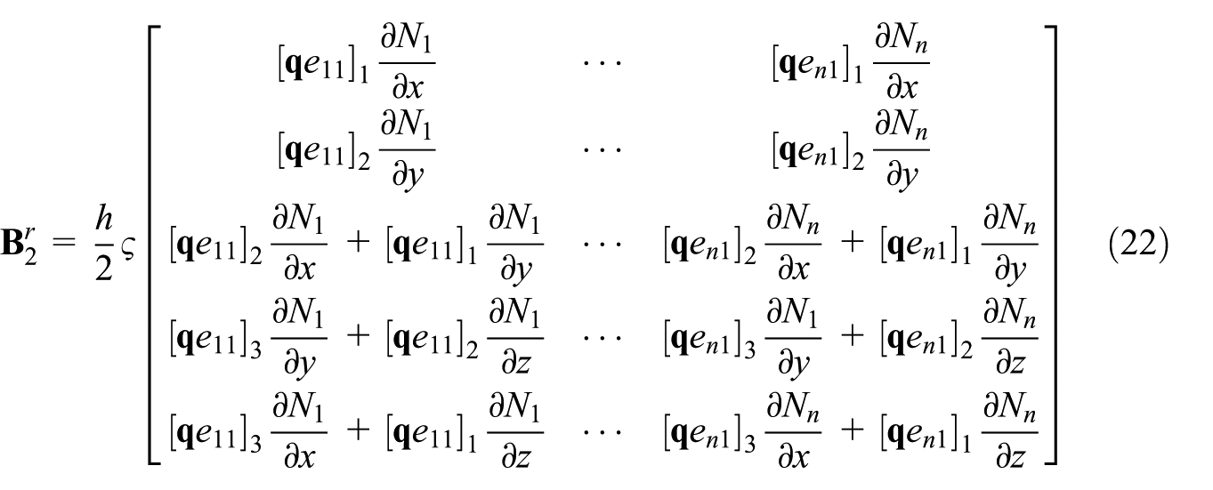
where h is the thickness of the shell. If the shell thickness is varying, it should appear as $h_A{N}_A$ in the content of the matrix in equations (21) and (22). $\mathbf{q}$ is the transformation matrix at a given quadrature point. ${\mathbf{e}}_{\mathrm{Ai}}$ is the $i\mathrm{th}$ local coordinate axis at the $A\mathrm{th}$ node. n is the number of basis functions whose value are non-zero at a given quadrature point. The calculation of the basis functions derivatives with respect to global coordinates can be obtained as in Hughes ³⁶ and Zhu et al. ³⁷

Finally, the contribution of a given quadrature point to the stiffness matrix is

$${\mathbf{K}}_q={{\mathbf{B}}_q}^T\mathbf{D}{\mathbf{B}}_q$$

(23)

where $\mathbf{D}$ is the modified material matrix and ${\mathbf{B}}_q$ is the strain-displacement matrix at the quadrature point, see Hughes. ³⁶ On multiplying the above contribution with its corresponding quadrature weight and then summing up on all quadrature points, we finally obtain the element stiffness matrix.

Isogeometric approximation with mixed grid

IGA uses the basis functions which are used in computer graphics and animation for analysis. This idea was first introduced by Hughes et al. ¹ using NURBS basis functions in the analysis. Following the success of this initial work, a lot of basis functions which are formerly used in CAD are used in IGA to extend its possibilities, such as T-spline, ³⁸ polynomial splines over hierarchical T-meshes (PHT) spline, ³⁹ and Hierarchical B-spline (HB). ⁴⁰ Considering that NURBS is the most common technology in the CAD society, we will use NURBS basis in this article. However, the extension to other basis functions mentioned previously is relatively straightforward. The definition of two-dimensional (2D) NURBS basis functions is as follows (see, for example, Piegl and Tiller ⁴¹ )

$$R_{i,j}^{p,q}=\frac{N_i^p\left(\xi \right)N_j^q\left(\eta \right)w_{\mathrm{ij}}}{\sum _{i=1}^n\sum _{j=1}^m{N}_i^p\left(\xi \right)N_j^q\left(\eta \right)w_{\mathrm{ij}}}$$

(24)

where $N^p$ and $N^q$ are one-dimensional (1D) B-spline basis functions which are defined by the knot vectors $\{{\xi }_1,{\xi }_2,\dots ,{\xi }_{n+p+1}\}$ and $\{{\eta }_1,{\eta }_2,\dots ,{\eta }_{n+p+1}\}$ . p and q are the degree of the 1D basis function in each parametric direction. n and m are the number of basis functions for each parametric direction, the total number of 2D basis function is $n\times m$ . $w_{\mathrm{ij}}$ are the weights of the control points and are driven by the geometric description of the 2D NURBS surface.

In IGA, once the description of the geometry is fixed, the coarsest mesh for analysis is obtained. After knot insertion and/or order elevation procedures, a finer mesh can be created without changing the geometry but only adding more basis functions and control points. This procedure is referred to as mesh refinement in IGA. ¹ The commonly used NURBS geometries in IGA are described by open knots vectors, which means that the first and end knots should appear $p+1$ times if the degree is p in the corresponding parametric direction. Each non-zero interval of the knot vector is defined as an element in 1D, in higher dimensions the tensor product structure is used to define the elements.

Introducing the basis functions of equation (24) into the shell model of the previous section, the isogeometric degenerated shell model can be devised. The starting point we consider here, as compared to what is done in finite element method (FEM) degenerated shells, is the definition of fiber vectors. Going back to the geometric description of the shell in equation (1) and considering a uniform shell, equation (1) can be rewritten as equation (25) and divided into two parts: the first one given in equation (26) is for the description of the mid-surface and the second one given in equation (27) is for the description of the director vectors

$$\mathbf{x}=\mathbf{s}+\mathbf{v}$$

(25)

$$\mathbf{s}=\sum _A{N}_A(\epsilon ,\eta ){\mathbf{x}}_A$$

(26)

$$\mathbf{v}=\frac{h}{2}\varsigma \sum _A{N}_A(\epsilon ,\eta ){\mathbf{y}}_A$$

(27)

The entire geometry can be viewed as the superposition of the mid-surface and the director field (see Figure 1).

Figure 1.

An example of $3\mathrm{D}$ shell shape description with NURBS basis and Lagrange basis. s is expressed with NURBS basis. Shell director v with linear Lagrange interpolation, basis points are the normal at points A, B, and C. Normals of points D and E are obtained by interpolation.

In traditional FEM, the fiber vectors ${\mathbf{y}}_A$ at each node can be naturally chosen as the normal of the shell at this node. The directors within the element can be found using equation (27). However, the control points in IGA do not belong to the represented geometry (except for piecewise linear NURBS which are identical to piecewise linear finite elements). As a consequence, there is no natural normal attached to the control points. Many methods have been proposed to fix this and define fiber vector at the node, as presented in the introduction. These methods need additional computational resources and programming effort. The problem when using the nearest point projection and taking the normal at the closest projected point as nodal values is that the approximation of the director vectors becomes worse as the polynomial order of the NURBS basis functions increases, see Figure 2 of Dornisch et al. ¹⁷ Dornisch et al. ¹⁷ proposed an approach that can exactly rebuild the directors at the quadrature points. It showed its superiority over the previous method. A preprocess is needed to extract the nodal directors, but such preprocess is used only one time, so its additional computation cost can be omitted in non-linear analysis where many iterations are often needed. Our approach to circumvent this is to use different representation for the thickness vectors $\mathbf{v}$ and the shell mid-surface $\mathbf{s}$ . Figure 1 shows the Lagrange interpolation of the shell directors and its superposition with the NURBS representation of the mid-surface to form the shape of the $3\mathrm{D}$ shell. Equation (26) is used to discretize $\mathbf{s}$ while equation (28) is used to discretize $\mathbf{v}$

$$\mathbf{v}=\frac{h}{2}\varsigma \sum _B{\hat{N}}_B(\epsilon ,\eta ){\mathbf{y}}_B$$

(28)

where ${\hat{N}}_B$ is the Lagrange basis. The “nodal” coordinates in parameter space are uniformly distributed in each element interval. There will exist $p_l+1$ basis points for p_l-order Lagrange basis functions, the first and end points will be located in the element interval’s end points. Their corresponding normal vectors in the NURBS mid-surface will be the basis ${\mathbf{y}}_B$ of equation (28). Their lamina coordinate systems will be used as nodal coordinate systems. An illustration of the mixed use of quadratic NURBS and quadratic Lagrange basis functions is depicted in Figure 2.

Figure 2.

An example of second-order Lagrange (slash lines), second-order NURBS basis functions, and the Lagrange basis points positions (squares) in IGA elements [ $0;0.3$ ] and [ $0.3;1$ ].

It should be noted that the Lagrange basis points are uniformly distributed in each IGA interval. Consequently, the value of the Lagrange basis function and their derivatives only need to be evaluated once in the isoparametric interval $[-1;1]$ . Then, to obtain the derivatives in an IGA interval of length l, multiplying them by $2/l$ allows us to obtain the correct value. The value of the Lagrange basis functions is kept unchanged in every interval. A similar approach can be used when implementing Gauss quadrature. From the above procedures, it can be seen that although we introduce additional Lagrange basis functions in our method, nearly no additional time and computational effort is spent on their evaluation. In a word, at the element level, if the same order rotational basis are used, our mixed approach needs roughly as much computational resources as the full NURBS approach. This credits to the scaling characteristics of the Lagrange basis functions.

Deriving the previous equations, the approximation of the deformation is also obtained using a combination of NURBS and Lagrange basis functions. The displacement of the shell given in equation (2) can be rewritten as

$$\mathbf{u}=\sum _A{N}_A(\epsilon ,\eta ){\mathbf{u}}_A+\frac{h}{2}\varsigma \sum _B{\hat{N}}_B(\epsilon ,\eta ){\mathbf{y}\mathbf{\text{'}}}_B$$

(29)

Following the derivation of the equation given in section “Degenerated shell model,” one can easily see that the expressions given in equations (20)–(22) are unchanged as long as the appropriate basis functions are used. That is, the NURBS basis functions N are used in equation (20), and the Lagrange basis functions $\hat{N}$ are used in equations (21) and (22). One can notice in the proposed approach that the concept of nodal degrees of freedom is not relevant as translational and rotational degrees of freedom are not associated to the same geometric points. In an isogeometric element, if we use degree $p_l$ Lagrange basis functions and degree $p\times q$ NURBS basis functions, there will be $3(p+1)(q+1)$ translational degrees of freedom and $2(p_l+1{)}^2$ rotational degrees of freedom. As for full structures of the same number of elements, if the basis of equal polynomial orders is used for full NURBS elements and our elements, our approach will give more degrees of freedom due to the lack of continuity in the Lagrange basis functions. This means that more computational resources will be needed to solve the structural linear equations. K Gauss quadrature points will be used with $K=\mathrm{maximum}(p,q,p_l)+1$ in each parametric direction.

Numerical examples

Three benchmark problems from shell obstacle courses of Belytschko et al. ⁴² and one double-curved free-form surface example taken from Dornisch et al. ¹⁷ are used here to validate our method and compare it with other isogeometric shell elements. In all the examples, we considered NURBS basis functions of degrees 2–5 and Lagrange basis functions of degrees 2 and 3. Increasing the degree of the Lagrange basis function does not improve the results when considering NURBS up to degree 5 as we will see in the sequel. In all cases, we use regular meshes with {2, 4, 8, 16, 32} elements per edges.

Scordelis–Lo roof problem

The problem setup and its material properties can be seen in Figure 3. A gravity load $g=90$ is applied to the model. The quantity of interest here is the vertical displacement $u_z$ at point A. The converged value is $-0.301969$ and is attained with $70\times 70$ elements mesh quartic NURBS $(P_N=4)$ and cubic Lagrange $(P_L=3)$ . It is comparable with the reference value $-0.3020247$ obtained by Dornisch et al. ¹⁷ using isogeometric Reissner–Mindlin shells with exactly calculated directors.

Figure 3.

Scordelis–Lo roof problem setup.

Figures 4 and 5 show the results with h refinement with various NURBS orders. Figure 4 shows the results obtained using quadratic Lagrange basis functions. For quadratic NURBS $P_N=2$ , the curves coincide with the results obtained with quadratic NURBS KL shells (developed by Kiendl et al. ¹² ). For cubic NURBS $P_N=3$ , the curve approaches the results obtained with cubic NURBS KL shells. For higher order NURBS $(P_N=4,5)$ , the results are not comparable with their corresponding KL shell results, but they are better than the ones obtained with $P_N=2,3$ . Figure 5 shows the results with the same NURBS polynomial order but using cubic Lagrange basis functions. All the curves coincide with those obtained using KL shells.

Figure 4.

Scordelis–Lo roof, $u_z$ versus number of elements per edges with quadratic Lagrange basis $(P_L=2)$ and various NURBS order.

Figure 5.

Scordelis–Lo roof, $u_z$ versus number of elements per edges with cubic Lagrange basis $(P_L=3)$ and various NURBS order.

Pinched cylinder problem

Figure 6 depicts the pinched cylinder problem setup and its material properties. Due to symmetry only one-eighth of the system is modeled and sketched. This example has been used by Dornisch et al. ¹⁷ to compare their exactly calculated director IGA shell with the KL shell of Kiendl et al. ¹² and the isogeometric Reissner–Mindlin shell of Benson et al. ¹³ The converged solution for the vertical displacement at point B is $1.85371\times {10}^{-5}$ with $32\times 32$ elements $P_N=5$ and $P_L=3$ . It is slightly different with the converged value $1.8248\times {10}^{-5}$ obtained by Dornisch et al., ¹⁷ but it is similar to the one obtained by Bouclier et al. ¹⁹ using a mesh of $32\times 32$ IGA solid shell elements $(1.85\times {10}^{-5})$ .

Figure 6.

Pinched cylinder with diaphragm problem setup.

Figures 7 and 8 depict the results obtained with h refinement with various NURBS orders. A similar behavior as for the previous example is observed. Figure 7 depicts the results obtained with quadratic Lagrange basis functions. The results of $P_N=2,3$ are comparable with these from KL shell. The results of $P_N=4,5$ are not comparable with these from KL shell, but they are better than $P_N=2,3$ . Figure 8 shows the results obtained with cubic Lagrange basis functions. The results of $P_N=2-4$ are closer to the converged line than those obtained by KL shell at the same mesh size. The result of $P_N=5$ approaches the one obtained with KL shell. A similar behavior when comparing the thick shell elements of Benson et al. ¹³ and Dornisch et al. ¹⁷ with KL shells results can be seen. Consequently, it can be observed that our approach leads to comparable results with these two alternative Reissner–Mindlin isogeometric shells. Figure 9 shows a direct comparison between our results and those from Benson et al. ¹³ and Dornisch et al. ¹⁷ All the results are normalized with $1.83\times {10}^{-5}$ . It can be seen clearly that for order 2–4, at the same mesh size, our results are closer to the reference line than the results obtained with two methods for this particular example.

Figure 7.

Pinched cylinder, $u_z$ versus number of elements per edges with quadratic Lagrange basis $(P_L=2)$ and various NURBS order.

Figure 8.

Pinched cylinder, $u_z$ versus number of elements per edges with cubic Lagrange basis $(P_L=3)$ and various NURBS order.

Figure 9.

Pinched cylinder, comparison of our approach with the one of Benson et al. ¹³ and Dornisch et al. ¹⁷ Present approach: $p=2$ indicates ( $P_N=2$ , $P_L=2$ ) and $p=3$ ( $P_N=3$ , $P_L=3$ ), $p=4$ ( $P_N=4$ , $P_L=3$ ).

Hemisphere shell problem

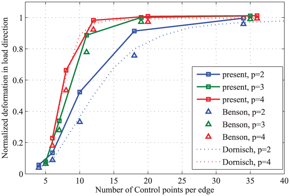
Figure 10 shows the hemisphere problem setup and its material properties. The quantity of interest is the horizontal displacement $u_x$ at point C. The converged solution is $0.0925$ with $32\times 32$ elements, $P_N=5$ and $P_L=3$ which is identical to the one found in the literature. Figures 11 and 12 show the convergence of the horizontal displacement at point C versus number of elements per edges using h refinement. The general behavior of our approach that was seen in the previous examples is again observed here.

Figure 10.

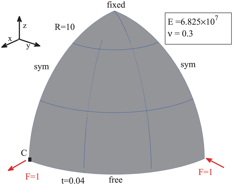
Hemisphere shell problem setup.

Figure 11.

Hemisphere shell, $u_x$ versus number of elements per edges with quadratic Lagrange basis $(P_L=2)$ and various NURBS order.

Figure 12.

Hemisphere shell, $u_x$ versus number of elements per edges with cubic Lagrange basis $(P_L=3)$ and various NURBS order.

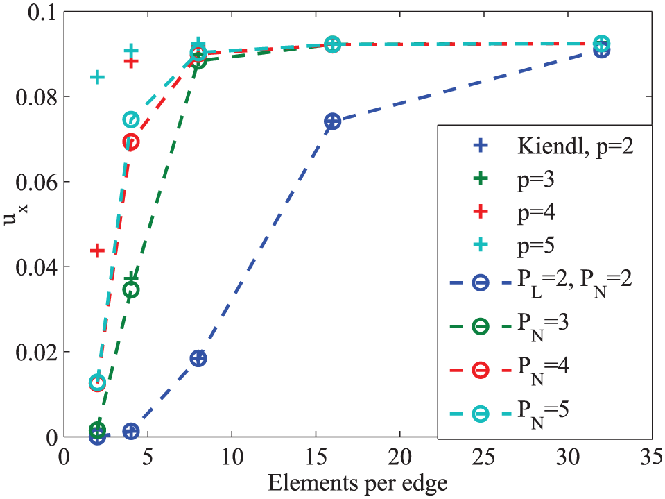
Double-curved free-form surface problem

This last example was designed by Dornisch et al. ¹⁷ to test their exactly calculated director IGA Reissner–Mindlin shell. Figure 13 shows the problem setup and material properties. The initial geometry description contains $3\times 3$ uniformly divided cubic elements. The quantity of interest is the horizontal displacement $u_y$ at point D, and the reference value is 1.02786 with $180\times 180$ NURBS elements with $p=6$ as reported in Dornisch et al. ¹⁷ We obtain 1.02529 as a converged value with $48\times 48$ elements $P_N=5$ and $P_L=3$ .

Figure 13.

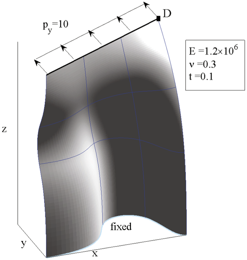
Double-curved free-form surface problem setup. Geometry data obtained from Dornisch et al. ¹⁷

Figure 14 shows the $u_y$ error variation around the reference value versus number of elements per edges with refined meshes obtained with h refinement. The curves labeled with “Benson” indicate that those results are obtained from shell elements, where the directors are interpolated following Benson’s approach. Our results are compared with the elements of Benson et al. ¹³ and Dornisch et al. ¹⁷ It can be seen that our results are not comparable with the ones obtained by Dornisch et al., ¹⁷ but they both approach the solution from the stiff side, whereas the results from the elements proposed by Benson et al. ¹³ approach it from the soft side. It should be noticed that we used cubic Lagrange basis functions to express the rotations for $P_N=4,5$ . This implies at the element level that there will be 32 rotational degrees of freedom in our method versus 50 $(p=4)$ and 72 $(p=5)$ with the standard methods. It decreases the time for building the stiffness matrix. But there are more degrees of freedom on the global scale. It will need more computational resources to solve the system equations.

Figure 14.

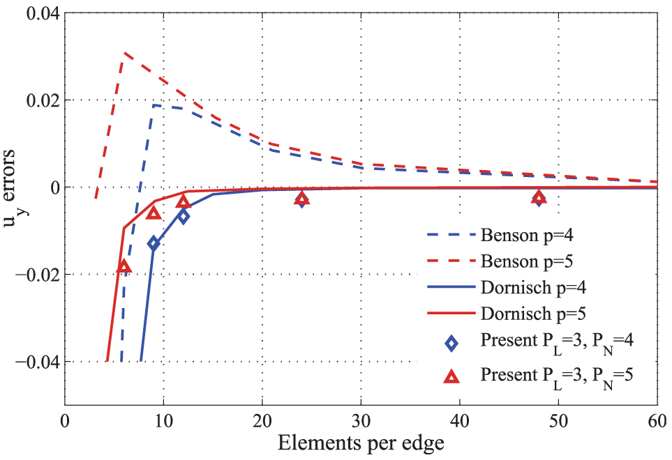
Double-curved free surface, $u_y$ variation with respect to the reference value $(u_y=1.02786)$ versus number of elements per edges. Results with alternative methods are taken from Dornisch et al. ¹⁷

Discussions

The results of different combinations of NURBS order and Lagrange order basis functions formulations all converge correctly. The differences lie in their convergence rates. This indicates the applicability of the independent formulation of the displacements and rotations in IGA shell elements. There can be different numbers of rotational and translational degrees of freedom in an element.

Figure 15 depicts an empirical estimation of the convergence rate performances of $P_N\mathrm{\&}{P}_L$ combinations. When $P_L>P_N$ , the results will be the same as the ones obtained for the same order, $P_L=P_N$ . For $P_L=1$ , using a NURBS order higher than $P_N=3$ does not improve the results. The red line we marked as “Good Performance” means that the corresponding results are comparable with the ones obtained with the same order $P_N$ and a NURBS KL shell. Thus, we suggest users to use these combinations. In other region, when increasing the values of $P_N$ or $P_L$ , the results (with the same numbers of elements) will improve. For instance, $P_L=2$ $P_N=3$ will produce better results than $P_L=2$ $P_N=2$ , and $P_L=3$ $P_N=3$ will likewise produce better results than $P_L=2$ $P_N=3$ . In the applications considered, we restricted ourselves to $P_L=[\begin{array}{ccc}\hfill 1,\hfill & \hfill 2,\hfill & \hfill 3\hfill \end{array}]$ and $P_N=[\begin{array}{ccccc}\hfill 1,\hfill & \hfill 2,\hfill & \hfill 3,\hfill & \hfill 4,\hfill & \hfill 5\hfill \end{array}]$ . We did not discuss the higher order NURBS and Lagrange basis cases, since we think that low-order elements might be privileged in engineering applications.

Figure 15.

Combination of NURBS basis orders and Lagrange basis orders.

As for the calculation efficiency, although we simultaneously use NURBS and Lagrange basis functions in our formulation, the additional cost of calculating the Lagrange basis function is relatively low. It indicates that our approach does not need more time to get the element stiffness matrices compared with the standard IGA shell. But on the global scale, our approach often gives more degrees of freedom especially when high-order basis are adopted; consequently, more computer resources will be needed to solve the system equations. However, when considering the case where $P_L<P_N$ , there will be fewer rotational basis functions compared with P_N-order full NURBS case, thus will to some extent ameliorate the above-mentioned problem. It is worth mentioning that there is no additional cost for the definition of fiber vectors in our method which is not the case for alternative isogeometric Reissner–Mindlin shells.^13,17 In another aspect, the method we proposed is a natural extension of the standard degenerated shell model, thus it is easy to implement compared with other IGA Reissner–Mindlin models.

Conclusion

In this article, we propose a new IGA Reissner–Mindlin shell formulation based on the mixed use of NURBS and Lagrange basis functions in the same domain. The use of NURBS basis functions to discretize the mid-surface of the shell keeps the geometry exact character of IGA analysis. The use of Lagrange basis avoids the determination of the director vectors commonly encountered in alternative IGA Reissner–Mindlin shell. Our method is a natural extension of standard degenerated Reissner–Mindlin shell, and it allows the use of traditional rotational boundary condition imposition technics, which is easier than that with full NURBS Reissner–Mindlin shells.

Our method does not need additional effort in the definition of fiber vectors, thus is easier to implement. It also allows the use of optimal or reduced quadrature rules, see for example, Hughes et al., ⁴³ Auricchio et al., ⁴⁴ and Schillinger et al., ⁴⁵ which can further reduce the calculation cost and/or improve the performance. Considering that the quadrature requirements in IGA analysis is different from that in FEM, ⁴³ new and general reduced quadrature strategies should be studied.