Sage Journals: Discover world-class research

Abstract

The vehicle is excited by the road surface while traveling. The vehicle suspensions play a significant role not only in damping out the vibrations created due to the excitation but also in maintaining the stability of the entire system. In this article, the dynamic stability of nonlinear suspension under this excitation is analyzed. The mathematic model for the suspension is established, the nonlinear vibration caused by sprung mass vibration is solved and frequency curves are obtained. Both the characteristics of the stable solution and the related parameters affecting the unstable region are analyzed. The numeric solution reveals the existence of a critical excitation value. When the excitation is within this critical value, the sprung mass vibration is stable; when the excitation is greater than the critical value, an unstable frequency band with the jumping phenomenon is observed. Under the same excitation acceleration, a decrease in damping coefficient results in an increase in both the amplitude and unstable frequency band, all falling into the unstable region which is getting larger. The increase in nonlinear stiffness of spring leads to the same maximum vibration amplitude shifting to the right and a larger unstable frequency band falling into the downward movement unstable region. All these indicate that there exists mutation in the amplitude of vehicle vibration, which endangers the stability of the vehicle while traveling.

Keywords

Nonlinear forced vibration internal resonance saddle node jumping phenomenon unstable region bifurcation

Introduction

Vehicle suspension system is a nonlinear vibration isolation system with 2 degrees of freedom. Its primary functions are to attenuate the vibration of sprung mass caused by road excitation and maintain the stability of the system.^1,2

To reduce the vibration acceleration of sprung mass as much as possible, researchers have carried out studies on the parameters of the system itself. In Febbo et al.,³ it has been found that the stronger the nonlinear characteristic of the primary isolation system, the better the vibration isolation effect of the system. Similar conclusions are reported in Lu et al.⁴ It has been found that the nonlinear term of the lower vibration isolation system can significantly affect the vibration isolation effect of the whole system. In Silveira et al.,⁵ an asymmetric nonlinear shock absorber is studied, which is reported as a better alternative to the linear absorber for vibration isolation. In the study of the single-degree-of-freedom oscillator, it has been found that when there are only cubic damping terms in the system without any linear terms, the nonlinear system has a better vibration isolation effect than its linear counterpart.⁶ In other studies, different road excitation effects on the system are analyzed in Petit et al.⁷ Several studies have focused on the robustness of the vibration isolation system.⁸ The performance of vibration isolation system with internal resonance has been analyzed in Ji.⁹ The vehicle seat vibration isolation system is also studied.^10,11 In the above studies, largely theoretical deduction, simulation analysis, and many results have been achieved. Also, the experiments are conducted, and the performance of the vibration isolation system is analyzed and verified further experimentally.^12–14

While ensuring a satisfactory vibration isolation performance, the system itself has the tendency of instability and should be avoided. The stability of magnetorheological fluid (MRF) isolation system is analyzed in Zhang et al.¹⁵ Elnaggar and Khalil¹⁶ and Ji¹⁷ presented the analysis on the stability of a single-degree-of-freedom vibration isolation system under secondary resonance. Literatures^18–20 focused on the stability of an oscillator under forced vibration. Jumping phenomenon is observed both theoretically and experimentally in the study of a nonlinear 2-degree-of-freedom vibration isolation system.²¹ Similar studies have been conducted in the literature; for instance, the stability analysis of seat isolation systems²² and the stability analysis of the high-speed railway suspension systems.²³

Many achievements have been made in these studies. However, the influence of system parameters on the stability is neglected while focusing on improving the efficiency of vibration isolation; in the studies focused on maintaining the stability of the system, the isolation effects are given less attention. The two studies are separated. The vehicle suspension system not only ensures good vibration isolation performance but also maintains the stability of the vehicle. Both of them need to be considered comprehensively. At the same time, in order to achieve a better vibration isolation effect, semi-active and active suspensions are introduced in literatures.^24–28 The stability of such a system is more crucial. Hence, more attention for this topic is worthy. Inspired by this, the stability of the suspension system is studied in this article ensuring the vibration isolation effect of the suspension system.

This article is organized as follows. In section “Mesoscopic model of closed-cell metallic foam,” the mathematical expression of one-fourth nonlinear suspension model is established and is solved using the method of multiple scales. The stability of the solution is analyzed in section “Dynamic response for the increasing density arrangement.” The proposed solution is validated in section “Dynamic response for the decreasing density arrangement” of this article. Section “Conclusion” concludes this article.

Governing equation for nonlinear suspension under forced vibration

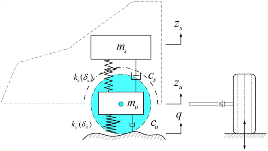
Leaving the turn of the vehicle out of account, the suspension model can be described as shown in Figure 1, which includes the sprung mass $m_{s}$ and the unsprung mass $m_{u}$ , connected by a nonlinear spring $k_{s}$ and a shock absorber $c_{s}$ . The wheel can be simplified as a nonlinear spring $k_{u}$ and a damper $c_{u}$ . When the automobile travels in the freeway, the construction vehicle crawls in the construction site or the military vehicle slows down preparing for a shooting, and the unevenness of the road is small, which is considered as q.

Figure 1.

Nonlinear quarter-car model.

According to Newton’s second law, the governing equations are as follows

m_{s} {\overset{\cdot\cdot}{z}}_{s} + f_{cs} ({\overset{\cdot}{z}}_{s} - {\overset{\cdot}{z}}_{u}) + f_{ks} (z_{s} - z_{u}) = 0

(1a)

\begin{array}{l} m_{u} {\overset{\cdot\cdot}{z}}_{u} - f_{c s} ({\dot{z}}_{s} - {\dot{z}}_{u}) - f_{k s} (z_{s} - z_{u}) \\ + f_{c u} ({\dot{z}}_{u} - \dot{q}) + f_{k u} (z_{u} - q) = 0 \end{array}

(1b)

where $f_{cs} ({\overset{\cdot}{z}}_{s} - {\overset{\cdot}{z}}_{u}) = c_{s} ({\overset{\cdot}{z}}_{s} - {\overset{\cdot}{z}}_{u})$ , $f_{ks} (z_{s} - z_{u}) = k_{s} (z_{s} - z_{u}) + δ_{s} (z_{s} - z_{u})^{3}$ , $f_{cu} ({\overset{\cdot}{z}}_{u} - \overset{\cdot}{q}) = c_{u} ({\overset{\cdot}{z}}_{u} - \overset{\cdot}{q})$ , and $f_{ku} (z_{u} - q) = k_{u} (z_{u} - q) + δ_{u} (z_{u} - q)^{3}$ .

The whole suspension is under a forced vibration state. Equations (1a) and (1b) can be changed as

\overset{\cdot\cdot}{x} + 2 ς_{x} w_{x} (\overset{\cdot}{x} - \overset{\cdot}{y}) + w_{x}^{2} (x - y) + β_{x} (x - y)^{3} = f \cos (Ω t)

(2a)

\begin{array}{l} \overset{\cdot\cdot}{y} - 2 ς_{x y} w_{x y} (\dot{x} - \dot{y}) - w_{x y}^{2} x - β_{x y} {(x - y)}^{3} \\ + 2 ς_{y} w_{y} \dot{y} + w_{y}^{2} y + β_{y} y^{3} = f \cos (Ω t) \end{array}

(2b)

where $z_{s} = x$ , $z_{u} = y$ , $w_{x}^{2} = k_{s} / m_{s}$ , $w_{xy}^{2} = k_{s} / m_{u}$ , $w_{y}^{2} = k_{s} + k_{u} / m_{u}$ , $ς_{x} = c_{s} / 2 w_{x} m_{s}$ , $ς_{xy} = c_{s} / 2 w_{xy} m_{u}$ , $ς_{y} = c_{u} / 2 w_{y} m_{u}$ , $β_{x} = δ_{s} / m_{s}$ , $β_{xy} = δ_{s} / m_{u}$ , $β_{y} = δ_{u} / m_{u}$ , and $- \overset{\cdot\cdot}{q} = f \cos (Ω t)$ . Here, $w_{x}$ and $w_{y}$ , $ς_{x}$ and $ς_{y}$ , and $β_{x}$ and $β_{y}$ denote the linearized natural frequencies, damping ratio, and nonlinear natural frequencies of sprung mass and unsprung mass, respectively. $w_{xy}$ , $ς_{xy}$ , and $β_{xy}$ are the natural frequencies, damping ratio, and nonlinear natural frequencies of unsprung mass caused by the spring $k_{s} (δ_{s})$ and the damper $c_{s}$ , respectively. $Ω$ is the excitation frequency.

The suspension mass varies due to the change of load. When $m_{s} \approx 9 m_{u} k_{s} / (k_{s} + k_{u})$ , the 3:1 internal resonance occurred.

Since the exact solution of equation (2) cannot be found, the method of multiple scales is applied in this article to solve this equation. A small perturbation parameter $ε$ is introduced, and the scale transformation is carried out.

In equation (2), the rate of change of the independent variable is much larger than that of the system, so that the system parameter can be transformed into a variable of slow time scale, as shown in equation (3)

\begin{array}{l} ς_{x} \to ε ς_{x}, ς_{x y} \to ε ς_{x y}, β_{x} \to ε β_{x}, \\ β_{x y} \to ε β_{x y}, w_{x y}^{2} x \to ε w_{x y}^{2} x, f \to ε f \end{array}

(3a)

ς_{y} \to ε^{2} ς_{y}, β_{y} \to ε^{2} β_{y}

(3b)

Since the stiffness of the tire $k_{u}$ is much higher, the nonlinearity term $δ_{u}$ is much smaller than that of the spring, and the equivalent damping coefficient $c_{u}$ is much smaller than the damper. The perturbation parameter is $ε^{2}$ (equation (3b)) when rescaling the stiffness and damping coefficient of the tire in the same equation.

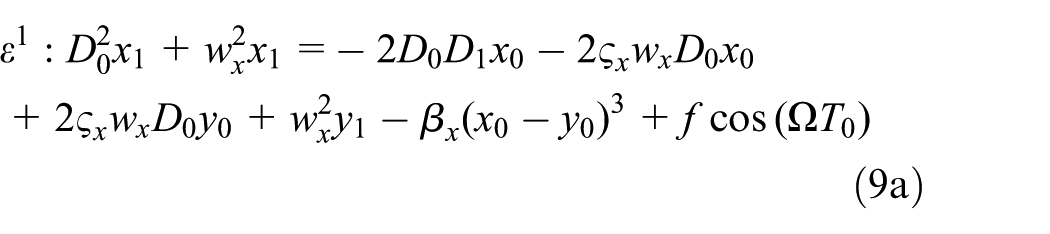
Substituting equation (3) into equation (2) and retaining the $ε^{0}$ and $ε^{1}$ terms yield the following equations

\begin{array}{l} \overset{\cdot\cdot}{x} + 2 ε ς_{x} w_{x} (\dot{x} - \dot{y}) + w_{x}^{2} (x - y) + ε β_{x} {(x - y)}^{3} \\ = ε f \cos (Ω t) \end{array}

(4a)

\begin{array}{l} \overset{\cdot\cdot}{y} - 2 ε ς_{x y} w_{x y} (\dot{x} - \dot{y}) - ε w_{x y}^{2} x - ε β_{x y} {(x - y)}^{3} + w_{y}^{2} y \\ = ε f \cos (Ω t) \end{array}

(4b)

The term $w_{xy}^{2} x$ in equation (2b) is much smaller in value than $w_{y}^{2} y$ , as such, this term can be considered as a small perturbation term. As a result of the above approximation, it can be rescaled as $ε w_{xy}^{2} x$ in equation (4b).

According to the method of multiscale, the approximate solution can be expressed as

x (t, ε) = x_{0} (T_{0}, T_{1}) + ε x_{1} (T_{0}, T_{1}) + O (ε^{2})

(5a)

y (t, ε) = y_{0} (T_{0}, T_{1}) + ε y_{1} (T_{0}, T_{1}) + O (ε^{2})

(5b)

where $T_{0} = t$ can be seen as a faster time scale and $T_{1} = ε t$ can be seen as a slower time scale.

Under 3:1 internal resonance condition

Ω = w_{x} + ε σ

(6a)

w_{y} = 3 w_{x} + ε σ_{2}

(6b)

where $σ$ is a detuning parameter expressing the closeness of $Ω$ to $w_{x}$ and $σ_{2}$ is a detuning parameter expressing the closeness of $w_{y}$ to $3 w_{x}$ .

There are differential operators like the following

\frac{d}{dt} (\cdot) = (D_{0} + ε D_{1}) (\cdot), \frac{d^{2}}{d t^{2}} (\cdot) = (D_{0}^{2} + 2 ε D_{0} D_{1}) (\cdot)

(7a)

D_{0} = \frac{\partial}{\partial T_{0}}, D_{1} = \frac{\partial}{\partial T_{1}}

(7b)

Substituting equations (5)–(7) into equation (4) and balancing similar terms of $ε$ results in the following equations

ε^{0} : D_{0}^{2} x_{0} + w_{x}^{2} x_{0} = w_{y}^{2} y_{0}

(8a)

ε^{0} : D_{0}^{2} y_{0} + w_{y}^{2} y_{0} = 0

(8b)

\begin{array}{l} ε^{1} : D_{0}^{2} x_{1} + w_{x}^{2} x_{1} = - 2 D_{0} D_{1} x_{0} - 2 ς_{x} w_{x} D_{0} x_{0} \\ + 2 ς_{x} w_{x} D_{0} y_{0} + w_{x}^{2} y_{1} - β_{x} {(x_{0} - y_{0})}^{3} + f \cos (Ω T_{0}) \end{array}

(9a)

\begin{array}{l} D_{0}^{2} y_{1} + w_{y}^{2} y_{1} = - 2 D_{0} D_{1} y_{0} - 2 ς_{x y} w_{x y} D_{0} y_{0} \\ + 2 ς_{x y} w_{x y} D_{0} x_{0} + {w_{x y}}^{2} x_{0} + β_{x y} {(x_{0} - y_{0})}^{3} + f \cos (Ω T_{0}) \end{array}

(9b)

The general solution of equation (8) can be expressed as follows

x_{0} = GB e^{i w_{y} T_{0}} + G \bar{B} e^{- i w_{y} T_{0}} + A e^{i w_{x} T_{0}} + \bar{A} e^{- i w_{x} T_{0}}

(10a)

y_{0} = B e^{i w_{y} T_{0}} + \bar{B} e^{- i w_{y} T_{0}}

(10b)

where amplitudes A and B are functions of slower time ( $T_{1}$ ), $\bar{A}$ and $\bar{B}$ are the complex conjugates of A and B, and $G = w_{x}^{2} / (w_{x}^{2} - w_{y}^{2})$ .

Substituting equation (10) into equation (9) and eliminating the secular terms results in the following equations

\begin{array}{l} - 2 A^{'} i w_{x} - 2 ς_{x} w_{x} A i w_{x} \\ - β_{x} [3 A^{2} \bar{A} + 6 A B \bar{B} {(G - 1)}^{2} + 3 {\bar{A}}^{2} B (G - 1) e^{i σ_{2} T_{1}}] \\ + \frac{1}{2} f e^{i σ T_{1}} = 0 \end{array}

(11a)

\begin{array}{l} - 2 B^{'} i w_{y} - 2 ς_{x y} w_{x y} B i w_{y} + 2 ς_{x y} w_{x y} G B i w_{y} + w_{x y}^{2} G B \\ + β_{x y} [6 A \bar{A} B (G - 1) + 3 B^{2} \bar{B} {(G - 1)}^{3} + A^{3} e^{- i σ_{2} T_{1}}] = 0 \end{array}

(11b)

Change A and B into polar form

A = \frac{1}{2} a e^{i β}

(12a)

B = \frac{1}{2} b e^{i θ}

(12b)

where a, b, $β$ , and $θ$ are the real functions of slower time ( $T_{1}$ ).

Substituting equation (12) into equation (11) and separating the real and imaginary parts yield the following equations

a' = - l_{1} a + h_{1} a^{2} b \sin (ϕ - 3 γ) - s_{2} \sin γ

(13a)

\begin{array}{l} a γ^{'} = - g_{1} a + h_{3} a^{3} + h_{2} a b^{2} \\ - h_{1} a^{2} b \cos (ϕ - 3 γ) - s_{2} \cos γ \end{array}

(13b)

b' = - l_{2} b + s_{1} a^{3} \sin (ϕ - 3 γ)

(13c)

b ϕ' = - g_{2} b + s_{3} b^{3} + s_{4} a^{2} b + s_{1} a^{3} \cos (ϕ - 3 γ)

(13d)

where $l_{1} = w_{x} ς_{x}$ , $h_{1} = - (3 / 8) (β_{x} / w_{x}) (G - 1)$ , $g_{1} = σ$ , $h_{2} = (3 / 4) (β_{x} / w_{x}) (G - 1)^{2}$ , $h_{3} = (3 / 8) (β_{x} / w_{x})$ , $l_{2} = ς_{xy} w_{xy} (1 - G)$ , $s_{1} = - (1 / 8) (β_{xy} / w_{y})$ , $s_{2} = (1 / 2) (f / w_{x})$ , $g_{2} = 3 σ - σ_{2} + (1 / 2) (w_{xy}^{2} / w_{y}) G$ , $s_{3} = - (3 β_{xy} / 8 w_{y}) (G - 1)^{3}$ , $s_{4} = - (3 / 4) (β_{xy} / w_{y}) (G - 1)$ , $γ = β - σ T_{1}$ , and $ϕ = θ + σ_{2} T_{1} - 3 σ T_{1}$ .

Stability analysis of solutions

The steady-state response of the system can be sought after eliminating the trigonometric terms in equation (13) by considering $a' = b' = 0$ and $γ' = ϕ' = 0$ . Then, bifurcation response of a and b can be expressed as follows

\begin{array}{l} s_{2}^{2} - l_{1}^{2} a^{2} + \frac{2 l_{2} l_{1} h_{1} b^{2}}{s_{1}} - h_{1}^{2} b^{2} a^{4} \\ - \frac{2 h_{1} (g_{1} - h_{2} b^{2} - h_{3} a^{2}) (g_{2} - s_{3} b^{2} - s_{4} a^{2}) b^{2}}{s_{1}} \\ - {(g_{1} - h_{2} b^{2} - h_{3} a^{2})}^{2} a^{2} = 0 \end{array}

(14a)

s_{1}^{2} a^{6} - l_{2}^{2} b^{2} - (g_{2} - s_{3} b^{2} - s_{4} a^{2})^{2} b^{2} = 0

(14b)

There are two kinds of solutions: uncoupled condition $a \neq 0$ , $b = 0$ and coupled condition $a \neq 0$ , $b \neq 0$ . As for the uncoupled condition, equation (14) can be simplified into the following form

s_{2}^{2} - l_{1}^{2} a^{2} - (g_{1} - h_{3} a^{2})^{2} a^{2} = 0

(15)

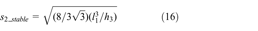
The number of solution concerned equation (15) can be 1 as well as 3. When the intensity of excitation from the road is beyond a certain value, the number of solutions is 3, resulting in the saddle-node bifurcation and jump phenomenon in the amplitude–frequency curve; when the intensity is within the critical value, only one solution can be sought. The critical value can be solved when there is only one solution for equation (15) throughout the whole frequency band

s_{2_stable} = \sqrt{(8 / 3 \sqrt{3}) (l_{1}^{3} / h_{3})}

(16)

As can be seen from equation (16), the critical value is related to the damping coefficient and nonlinearity stiffness of the spring.

Combining equations (6), (10), and (12), one can obtain the following

x = Gb \cos (3 Ω t + ϕ) + a \cos (Ω t + γ) + O (ε)

(17a)

y = b \cos (3 Ω t + ϕ) + O (ε)

(17b)

From equation (17), one can see that in coupled condition, there exist two vibration frequency, that is, forced vibration frequency $Ω$ and free vibration frequency $3 Ω$ due to the existence of internal resonance. The nonlinear stiffness of the spring makes the free vibration frequency exactly three times that of the forcing frequency. As for the uncoupled conditions, the vehicle vibration is mainly reflected by the vibration of sprung mass, and there is only one vibration frequency in the vehicle.

When the suspension is in the uncoupled condition, the steady state of sprung mass vibration is that of the autonomous system in the singularity $(\bar{a}, \bar{r})$ . Linearize the system.

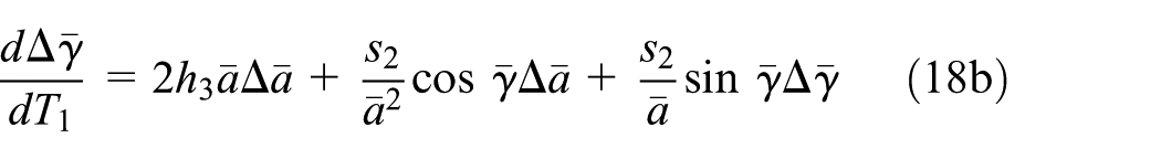
Linearizing equations (13a) and (13b) in the singularity $(\bar{a}, \bar{r})$ yields the following equations about disturbance of $Δ \bar{a}$ and $Δ \bar{r}$ : (The linearization process includes $(\bar{a})' = 1 \cdot Δ \bar{a}$ , $({\bar{a}}^{2})' = 2 \bar{a} \cdot Δ \bar{a}$ , $(\sin \bar{r})' = \cos \bar{r} Δ \bar{r}$ , and $(\cos \bar{r} / a)' = - (\sin \bar{r} Δ \bar{r} \bar{a} - \cos \bar{r} Δ \bar{a}) / {\bar{a}}^{2}$ .)

\frac{d Δ \bar{a}}{d T_{1}} = - l_{1} Δ \bar{a} - s_{2} \cos \bar{γ} Δ \bar{γ}

(18a)

\frac{d Δ \bar{γ}}{d T_{1}} = 2 h_{3} \bar{a} Δ \bar{a} + \frac{s_{2}}{{\bar{a}}^{2}} \cos \bar{γ} Δ \bar{a} + \frac{s_{2}}{\bar{a}} \sin \bar{γ} Δ \bar{γ}

(18b)

Using $a' = γ' = 0$ to eliminate $\bar{γ}$ in the above equation, the following equation can be obtained

det [\begin{matrix} \begin{matrix} - l_{1} w_{x} - λ \\ M \end{matrix} & \begin{matrix} N \\ - l_{1} w_{x} - λ \end{matrix} \end{matrix}] = 0

(19)

where $M = 1 / \bar{a} [- g_{1} w_{x} + 3 h_{3} w_{x} {\bar{a}}^{2}]$ and $N = - \bar{a} [- g_{1} w_{x} + h_{3} w_{x} {\bar{a}}^{2}]$ .

Expand equation (19)

λ^{2} + 2 λ l_{1} w_{x} + l_{1}^{2} w_{x}^{2} + w_{x}^{2} g_{1}^{2} - 4 h_{3} {\bar{a}}^{2} w_{x}^{2} g_{1} + 3 h_{3}^{2} {\bar{a}}^{4} w_{x}^{2} = 0

(20)

The solution to equation (20) is

λ_{1, 2} = \frac{1}{2} (- P \pm \sqrt{P^{2} - 4 Q})

(21)

where $P = 2 l_{1} w_{x}$ and $Q = l_{1}^{2} w_{x}^{2} + w_{x}^{2} g_{1}^{2} - 4 h_{3} {\bar{a}}^{2} w_{x}^{2} g_{1} + 3 h_{3}^{2} {\bar{a}}^{4} w_{x}^{2}$ .

When $P > 0$ and $Q < 0$ , $λ_{1, 2}$ is the real eigenvalue and $λ_{1} λ_{2} < 0$ . At this moment, the steady-state solution is unstable. In other words, as for $l_{1} > 0$ , the condition of losing stability for steady-state solution is

l_{1}^{2} + g_{1}^{2} - 4 h_{3} {\bar{a}}^{2} g_{1} + 3 h_{3}^{2} {\bar{a}}^{4} < 0

(22)

Therefore, the solution set to this equation constitutes the unstable region. The rest is stable region. The solving process can be done in MATLAB.

Numerical validation

Analysis of frequency response

When $m_{s} = 45 kg$ , $m_{u} = 45 kg$ , $k_{s} = 2000 N / m$ , $δ_{s} = 660 N / m$ , $k_{u} = 16, 000 N / m$ , and $c_{s} = 20 N s / m$ , then $w_{y} = 20 rad / s$ , $w_{x} = 6.6667 rad / s$ , and $w_{y} \approx 3 w_{x}$ .

According to equation (16), the maximum excitation acceleration for which the bifurcation does not occur in the steady state is $f_{stable} = 2 w_{x} s_{2_stable} = 1.9081 m / s^{2}$ . When the excitation acceleration increases, the amplitude of the sprung mass vibration will appear to bifurcate due to the saddle node, that is, jumping phenomenon in the amplitude–frequency curve.

It can be seen from Figure 2 that when the excitation acceleration is less than $f_{stable}$ , the amplitude–frequency curve is single-valued and remains the same during the forward frequency sweep or backward frequency sweep. When the excitation acceleration is much higher than $f_{stable}$ , jumping phenomenon occurs. When the frequency is swept up, the amplitude continues to increase to the top and then drop down to a much lower level. As the frequency continues to increase, the amplitude declines. When the frequency is swept down, the opposite jump up phenomenon will occur. In another word, the amplitude–frequency curve shows the jumping phenomenon due to the bifurcation. The curve is different during the forward frequency sweep and backward frequency sweep. With the increase in excitation acceleration, the vibration amplitude of the sprung mass of all frequency bands increases and the unstable frequency band increases.

Figure 2.

The effect of varying acceleration f on frequency response of vibration a: $f = 1 m / s^{2}$ (black squares), $f = 3 m / s^{2}$ (red triangles), $f = 5 m / s^{2}$ (blue crosses), and $f = 7 m / s^{2}$ (green dots).

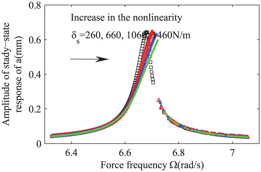
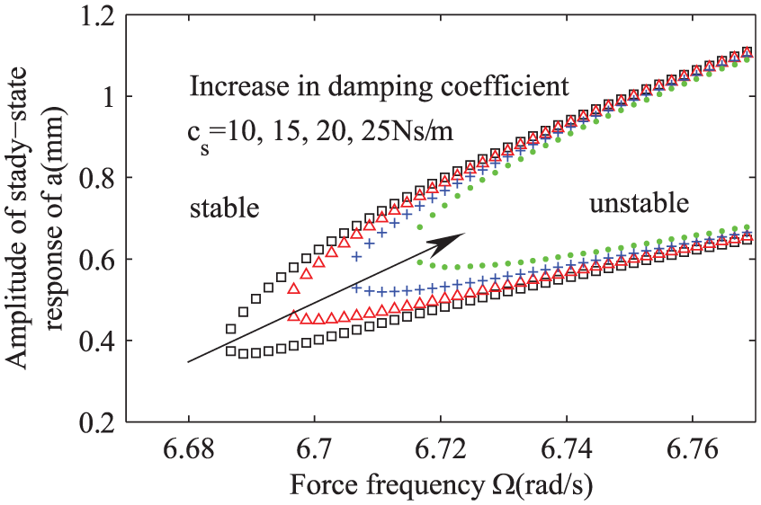
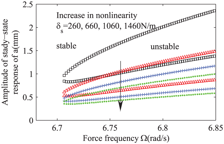
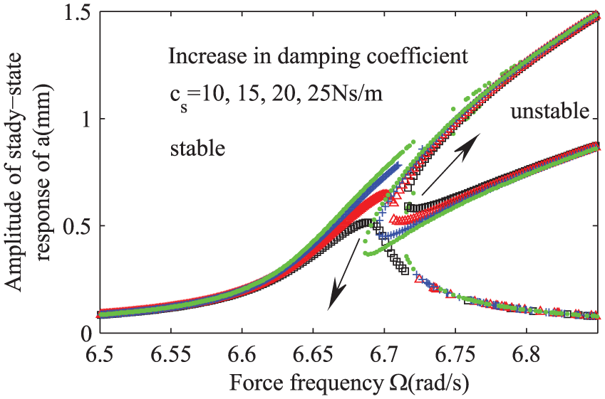
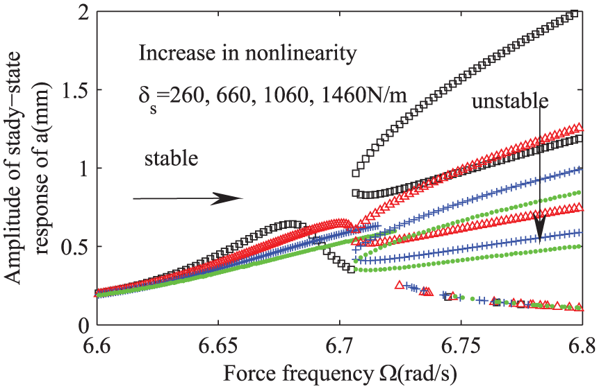
Figures 3 and 4 are frequency response curves for $δ_{s} = 660 N / m$ and $c_{s} = 20 N s / m$ , respectively, and $f_{stable} = 1.9081 m / s^{2}$ in Figures 3 and 4. It can be seen in Figure 3 that when the damping coefficient of the damper is higher than $20 N s / m$ , in which case the solution is stable, the steady-state solution of the sprung mass vibration does not bifurcate. On the contrary, bifurcation occurs in the steady-state solution of the sprung mass vibration, and the smaller the damping coefficient is, the wider the unstable bands become. Unlike the results in Figure 2, only the amplitude of the frequency that is closer to the resonant frequency will get larger as the damping coefficient decreases. The changes at remaining frequencies are negligible. This clearly indicates that decreasing the damping coefficient has a significant effect on the amplitude of the frequency which is close to the resonant frequency, enlarging both the amplitude and the unstable frequency bands. In the rest of the frequency band, the amplitude has nothing to do with the damping coefficient. Figure 4 shows that the nonlinearity of the spring does not increase the vibration amplitude of the sprung mass, but causes the resonance point to shift to the right and generates unstable bands. It can be concluded from Figures 2 to 4 that increasing the excitation acceleration, decreasing the damping coefficient of the damper, and increasing the nonlinearity of the spring will result in a wider and wider unstable frequency bands.

Figure 3.

The effect of varying damping coefficient $c_{s}$ on frequency response of vibration a: $c_{s} = 25 N s / m$ (black squares), $c_{s} = 20 N s / m$ (red triangles), $c_{s} = 15 N s / m$ (blue crosses), and $c_{s} = 10 N s / m$ (green dots).

Figure 4.

The effect of varying nonlinearity $δ_{s}$ on frequency response of vibration a: $δ_{s} = 260 N / m$ (black squares), $δ_{s} = 660 N / m$ (red triangles), $δ_{s} = 1060 N / m$ (blue crosses), and $δ_{s} = 1460 N / m$ (green dots).

From Figure 2, it can be found that when the amplitude–frequency curve shows an unstable frequency band, the excitation acceleration and force–frequency will appear at multiple values. This is reflected more clearly in Figure 5 when $c_{s} = 20 Ns / m$ and $δ_{s} = 660 N / m$ are considered. In a smaller force frequency like $Ω = 6.67 rad / s$ and $Ω = 6.72 rad / s$ , the amplitude of the sprung mass vibration is a single-valued curve; when $Ω = 6.77 rad / s$ and $Ω = 6.82 rad / s$ , the curve changes to multi-valued curve. Similar to Figure 2, in the multi-value curve, there is a jumping phenomenon in the process of increasing or decreasing the excitation acceleration, and the acceleration response curve is different. As a result, the force frequency becomes higher and the unstable interval of the excitation acceleration gets wider and gradually shifts to the right. Unlike Figure 2, with a small excitation acceleration, the amplitude decreases as the force frequency increases; with a higher excitation acceleration, the opposite will occur.

Figure 5.

The effect of varying force frequency $Ω$ on force acceleration response of vibration a: $Ω = 6.67 rad / s$ (black squares), $Ω = 6.72 rad / s$ (red triangles), $Ω = 6.77 rad / s$ (blue crosses), and $Ω = 6.82 rad / s$ (green dots).

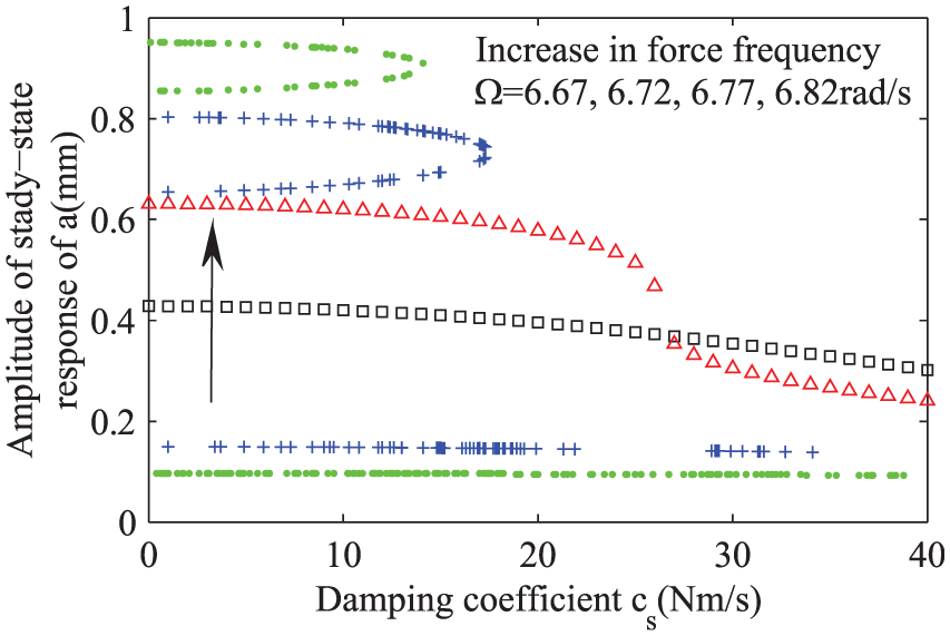
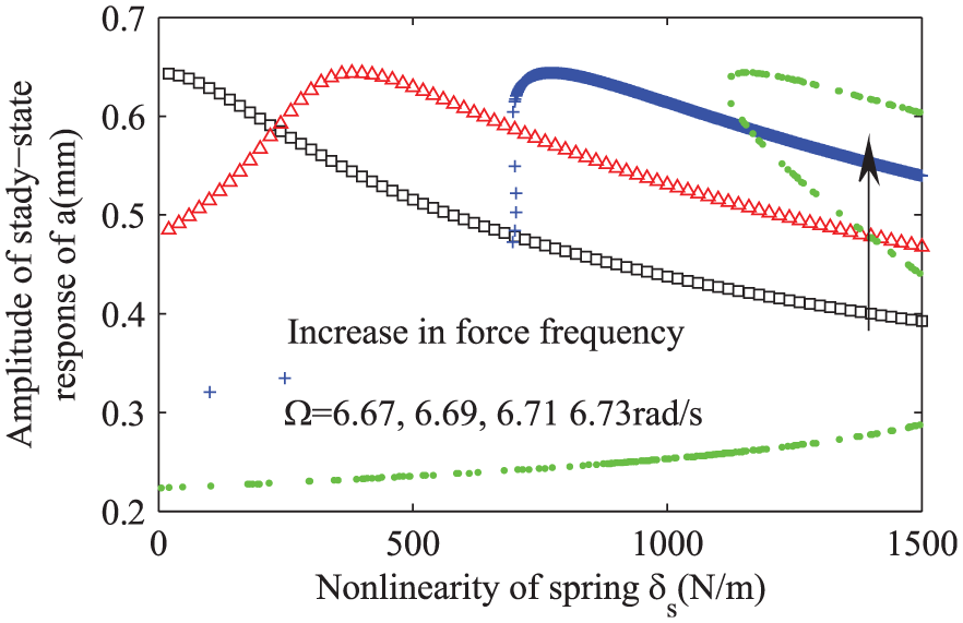
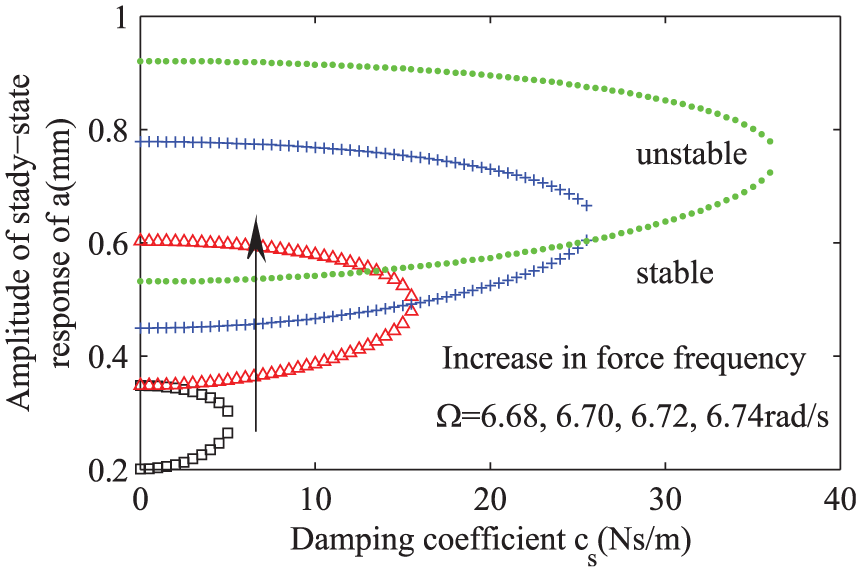
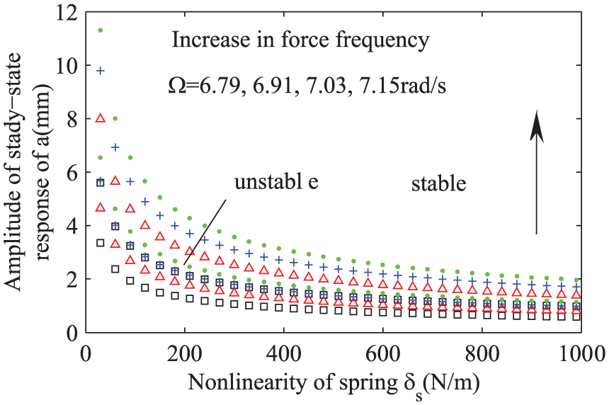
Figures 6 and 7 are the frequency response curves when $δ_{s} = 660 N / m$ and $c_{s} = 20 N s / m$ , respectively, and $f_{stable} = 1.9081 m / s^{2}$ in both the cases. It can be seen in Figure 6 that for a small force frequency like $Ω = 6.67 rad / s$ and $Ω = 6.72 rad / s$ , the amplitude of the sprung mass vibration is a single-valued curve, which decreases as the damping coefficient increases. When $Ω = 6.77$ and $6.82 rad / s$ , the curve changes to multi-valued curve. In the process of increasing the damping coefficient, the unstable damping coefficient interval under small force frequency gradually moves to the right and decreases, and curves converge in the end. Figure 7 shows that when the nonlinear stiffness of the spring increases, the higher the force frequency, the larger the vibration amplitude, and the unstable nonlinear stiffness interval increases and shifts to the right. However, the maximum amplitude of the sprung mass vibration in the whole nonlinear stiffness range is equal.

Figure 6.

The effect of varying force frequency $Ω$ on damping coefficient response of vibration a: $Ω = 6.67 rad / s$ (black squares), $Ω = 6.72 rad / s$ (red triangles), $Ω = 6.77 rad / s$ (blue crosses), and $Ω = 6.82 rad / s$ (green dots).

Figure 7.

The effect of varying force frequency $Ω$ on nonlinearity response of tire vibration a: $Ω = 6.67 rad / s$ (black squares), $Ω = 6.72 rad / s$ (red triangles), $Ω = 6.77 rad / s$ (blue crosses), and $Ω = 6.82 rad / s$ (green dots).

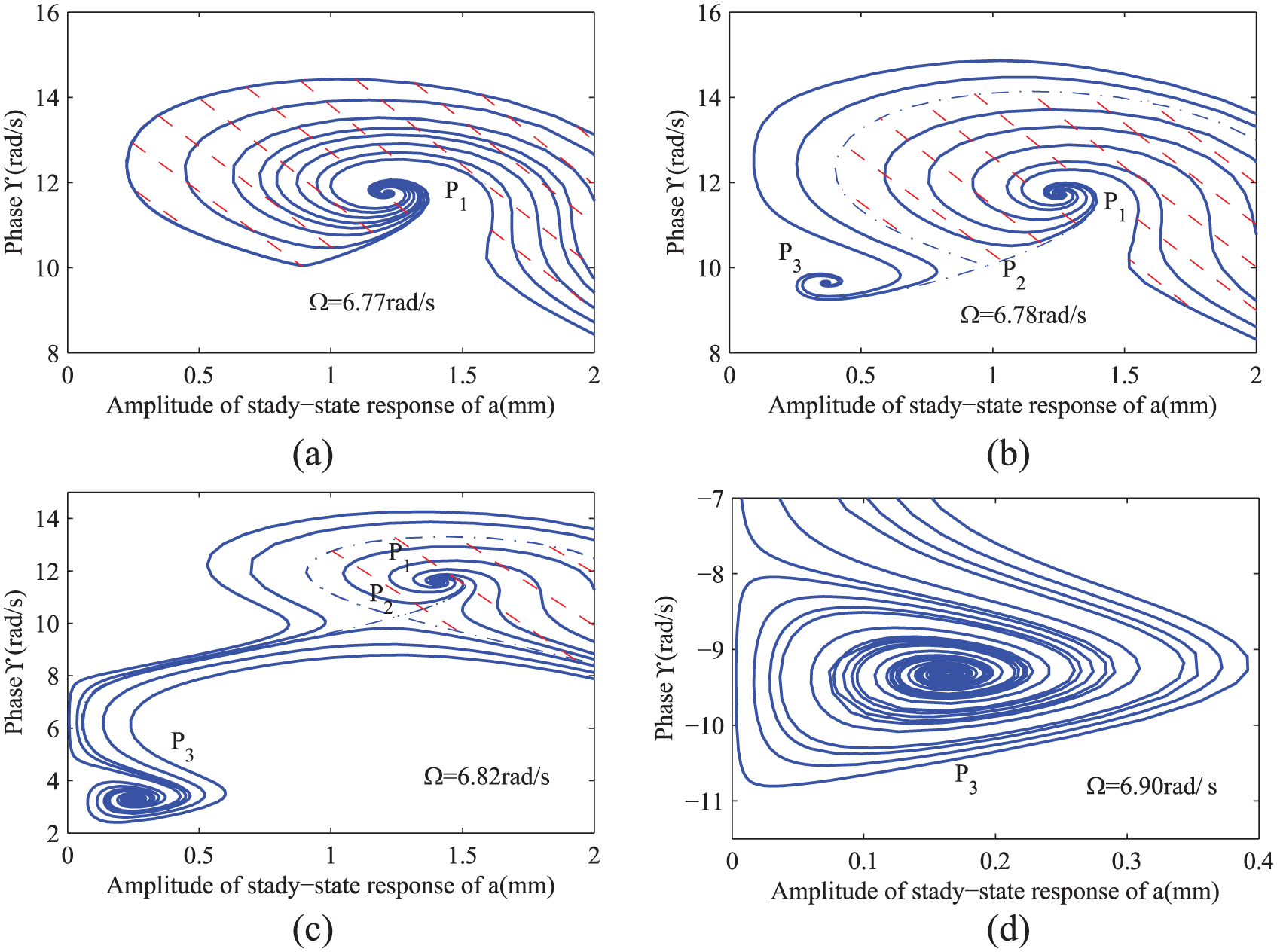
To better illustrate the stability of the solution and the jumping phenomenon in the frequency response curve, consider the value of $σ$ that falls in the interval in which the frequency response curve is a multi-valued curve. For the nonlinear system, the solution of the forced vibration is related to the initial conditions, and every time there is more than one stable steady-state solution, the initial condition determines which solution will occur in the actual physical world. Calculating and drawing the state plane trajectory under different initial conditions with the integral of equations (13a) and (13b) ( $b = 0$ ), one can obtain Figure 8.

Figure 8.

Evolution of the phase plane with the force frequency: (a) 6.77, (b) 6.78, (c) 6.82, and (d) 6.90 rad/s.

The critical lower limit frequency is $w_{down}$ and the critical upper limit frequency is $w_{upper}$ . When the force frequency $Ω$ gets close to $w_{down}$ , all vibrations under different initial conditions are attracted to the stable focus $P_{1}$ . Once the force frequency $Ω$ satisfies $Ω > w_{down}$ , another stable focus $P_{3}$ is generated, which is shown in Figure 8(a) and (b). It can be seen in Figure 8(c) that when the force frequency $Ω$ satisfies $w_{down} < Ω < w_{upper}$ , there exist only two stable focuses $P_{1}$ and $P_{3}$ and a saddle node $P_{2}$ . Only certain initial conditions can lead to a trajectory which can get to the saddle node $P_{2}$ . With a small disturbance, the system state will be attracted to focus $P_{1}$ or $P_{3}$ . The dotted line in Figure 8(c) is the dividing line between the two regions. The state outside the dotted line is attracted to the stable focus $P_{3}$ and that inside the dotted line is attracted to the stable focus $P_{1}$ . As the force frequency continues to increase, at time $Ω > w_{upper}$ , the focus $P_{1}$ disappears, and all states are attracted to the focus $P_{3}$ . The region covered by red dashed line varies from large to small and ultimately disappears. This phenomenon indicates that the upper and the lower two solutions are asymptotically stable in the amplitude–frequency curve, and the intermediate solution is unstable. As the asymptotically stable motion can be achieved in the actual physical world, the jumping phenomenon can be observed.

Change of the unstable region

In section “Dynamic response,” the characteristics of the unstable solution of sprung mass vibration have been analyzed, and the regional range of unstable solution is focused here.

Considering the damping coefficient $δ_{s} = 660 N / m$ and the nonlinear stiffness $c_{s} = 20 N s / m$ , Figures 9 and 10 are obtained. It can be seen in Figure 9 that with an increase in the damping coefficient, the unstable region is reduced along the direction of the saddle node. As the damping coefficient increases, the amplitude of the amplitude–frequency curve decreases. Hence, the number of solutions of the frequency response curve that falls in the unstable region decreases and the system stability increases. Similar to Figure 9, as the nonlinear stiffness increases, the whole unstable region in Figure 10 is reduced and gradually moves down. As the nonlinear stiffness increases, the peak amplitude of frequency curve gradually moves to the right. Although the unstable area decreases, the downward movement means that the amplitude–frequency curve will appear as unstable intermediate solution; therefore, the stability of the system is weak.

Figure 9.

The effect of varying the damping coefficient $c_{s}$ on unstable area of vibration a: $c_{s} = 10 N s / m$ (black squares), $c_{s} = 15 N s / m$ (red triangles), $c_{s} = 20 N s / m$ (blue crosses), and $c_{s} = 25 N s / m$ (green dots).

Figure 10.

The effect of varying the nonlinearity $δ_{s}$ on unstable area of vibration a: $δ_{s} = 260 N / m$ (black squares), $δ_{s} = 660 N / m$ (red triangles), $δ_{s} = 1060 N / m$ (blue crosses), and $δ_{s} = 1460 N / m$ (green dots).

Considering the damping coefficient $δ_{s} = 660 N / m$ and the nonlinear stiffness $c_{s} = 20 N s / m$ , Figures 11 and 12 are obtained. Figures 11 and 12 indicate that in the whole range of damping coefficient, as the force frequency increases, the unstable region increases and moves to the upper right. At this point, the unstable intermediate solutions in Figure 6 fall into the unstable region, and the number of unstable solutions increases, and the system stability becomes weaker. The nonlinear stiffness increases and the area of the unstable region increases. At this point, the unstable intermediate solutions in Figure 7 fall into the unstable region, and the number of unstable solutions increases and the system stability becomes weaker. To better illustrate the relationship between the unstable region and the amplitude–frequency curve, the amplitude–frequency curve and the unstable region are compared in the same figure, and Figures 13 and 14 are obtained.

Figure 11.

The effect of varying force frequency $Ω$ on the unstable area of vibration a: $Ω = 6.68 rad / s$ (black squares), $Ω = 6.70 rad / s$ (red triangles), $Ω = 6.72 rad / s$ (blue crosses), and $Ω = 6.74 rad / s$ (green dots).

Figure 12.

The effect of varying force frequency $Ω$ on the unstable area of vibration a: $Ω = 6.79 rad / s$ (black squares), $Ω = 6.91 rad / s$ (red triangles), $Ω = 7.03 rad / s$ (blue crosses), and $Ω = 7.15 rad / s$ (green dots).

Figure 13.

The effect of varying damping coefficient $c_{s}$ on frequency response (unstable area) of vibration a: $c_{s} = 10 N s / m$ (black squares), $c_{s} = 15 N s / m$ (red triangles), $c_{s} = 20 N s / m$ (blue crosses), and $c_{s} = 25 N s / m$ (green dots).

Figure 14.

The effect of varying nonlinearity $δ_{s}$ on frequency response (unstable area) of vibration a: $δ_{s} = 260 N / m$ (black squares), $δ_{s} = 660 N / m$ (red stars), $δ_{s} = 1060 N / m$ (blue crosses), and $δ_{s} = 1460 N / m$ (green dots).

It can be seen from Figures 13 and 14 that the band in which the jumping phenomenon occurs in the amplitude–frequency curve is located in the unstable region. The damping coefficient decreases, the amplitude of the amplitude–frequency curve increases, the unstable frequency band increases, and the number of unstable solutions (intermediate solution branches) increases. At the same time, the area of the unstable region becomes larger, and the intermediate solution branches fall into the unstable region. Thus, the system stability weakens with the decrease in the damping coefficient. With the increase in nonlinear stiffness, the frequency band of the amplitude–frequency curve is shifted to the right. Although the instability area decreases, the downward movement implies the emergence of unstable intermediate solutions in the amplitude–frequency curve, and the solution falls in this unstable region, and the system stability is weakened. This is consistent with the analysis of the previous results.

Conclusion

Vehicle suspension is a nonlinear system with 2 degrees of freedom. The vehicle is excited by the road surface while traveling. When the unsprung quality $m_{u}$ , sprung mass $m_{s}$ , the linear stiffness of tire $k_{u}$ , and the linear stiffness of the suspension spring $k_{s}$ satisfy the condition $m_{s} \approx 9 m_{u} k_{s} / (k_{s} + k_{u})$ , the vibration frequency ratio of unsprung mass and sprung mass is 3:1, and internal resonance will occur. Under the condition of internal resonance, when the sprung mass and the unsprung mass are not coupled, the vibration amplitude of the sprung mass exhibits a jumping phenomenon. This mutation amplitude may endanger the route judgment of the self-piloting automobile or cause missing target when shooting in case of the military vehicles, which is worthy of further study.

The analysis results show that there exists a critical value of excitation when the damping coefficient of the damper and the stiffness of the suspension spring are constant. When the value of the excitation is within this critical value, the sprung mass vibration is stable; when the excitation is larger than the critical value, the unstable frequency band with the jumping phenomenon occurs. Moreover, under the same excitation acceleration, the decrease in damping coefficient results in an increase both in amplitude and unstable frequency band, all falling into an unstable region, which is getting larger. The increase in nonlinear stiffness of spring leads to the same maximum vibration amplitude shifting to the right and a larger unstable frequency band falling into the downward movement unstable region. All these indicate that there exists mutation in the amplitude of vehicle vibration, which endangers the stability of the vehicle while traveling.

Footnotes

Handling Editor: Crinela Pislaru

Declaration of conflicting interests

The author(s) declared no potential conflicts of interest with respect to the research, authorship, and/or publication of this article.

Funding

The author(s) received no financial support for the research, authorship, and/or publication of this article.

ORCID iD

Jun Yao

References

Acar

Yilmaz

Design of an adaptive–passive dynamic vibration absorber composed of a string–mass system equipped with negative stiffness tension adjusting mechanism. J Sound Vib 2013; 332: 231–245.

Yao

JH.

Hopf bifurcation for a model of cellular shock instability. Physica D 2014; 269: 63–75.

Febbo

Machado

SP.

Nonlinear dynamic vibration absorbers with a saturation. J Sound Vib 2013; 332: 1465–1483.

Brennan

Yang

et al . An investigation of a two-stage nonlinear vibration isolation system. J Sound Vib 2013; 332: 1456–1464.

Silveira

Pontes

Jr Balthazar

JM.

Use of nonlinear asymmetrical shock absorber to improve comfort on passenger vehicles. J Sound Vib 2014; 333: 2114–2129.

Xiao

Jing

Cheng

The transmissibility of vibration isolators with cubic nonlinear damping under both force and base excitations. J Sound Vib 2013; 332: 1335–1354.

Petit

Loccufier

Aeyels

The energy thresholds of nonlinear vibration absorbers. Nonlinear Dynam 2013; 74: 755–767.

Detrouxn

Habib

Masset

et al . Performance, robustness and sensitivity analysis of the nonlinear tuned vibration absorber. Mech Syst Signal Pr 2015; 60–61: 799–809.

JC.

Design of a nonlinear vibration absorber using three-to-one internal resonances. Mech Syst Signal Pr 2014; 42: 236–246.

10.

Sun

Jing

XJ.

Analysis and design of a nonlinear stiffness and damping system with a scissor-like structure. Mech Syst Signal Pr 2016; 66–67: 723–742.

11.

Gao

Chen

Liu

XB.

Nonlinear dynamics and design for a class of piecewise smooth vibration isolation system. Nonlinear Dynam 2016; 84: 1715–1726.

12.

Ahn

KK.

Experimental investigation of a vibration isolation system using negative stiffness structure. Int J Mech Sci 2013; 70: 90–112.

13.

Araki

Asai

Kimura

et al . Nonlinear vibration isolator with adjustable restoring force. J Sound Vib 2013; 332: 6063–6077.

14.

Tang

Brennan

Gatti

et al . Experimental characterization of a nonlinear vibration absorber using free vibration. J Sound Vib 2016; 367: 159–169.

15.

Zhang

Min

et al . Bifurcations and chaos of a vibration isolation system with magneto-rheological damper. AIP Adv 2016; 6: 035310.

16.

Elnaggar

Khalil

KM.

Control of the nonlinear oscillator bifurcation under superharmonic resonance. J Appl Mech Tech Phy 2013; 54: 34–43.

17.

JC.

Secondary resonances of a quadratic nonlinear oscillator following two-to-one resonant Hopf bifurcations. Nonlinear Dynam 2014; 78: 2161–2184.

18.

Andreaus

Casini

Dynamics of friction oscillators excited by a moving base and/or driving force. J Sound Vib 2001; 245: 685–699.

19.

Andreaus

De Angelis

Nonlinear dynamic response of a base-excited SDOF oscillator with double-side unilateral constraints. Nonlinear Dynam 2016; 84: 1447–1467.

20.

Yang

Xiong

Xing

JT.

Power flow behaviour and dynamic performance of a nonlinear vibration absorber coupled to a nonlinear oscillator. Nonlinear Dynam 2015; 80: 1063–1079.

21.

Djemal

Chaari

Dion

J-L

et al . Performance of a non linear dynamic vibration absorbers. J Mech 2014; 31: 345–353.

22.

Yan

Zhu

et al . Modeling and analysis of static and dynamic characteristics of nonlinear seat suspension for off-road vehicles. Shock Vibr 2015; 2015: 938205.

23.

Zhang

Dai

HY.

Bifurcation analysis of high-speed railway wheel-set. Nonlinear Dynam 2016; 83: 1511–1528.

24.

Nguyen

Choi

S-B.

A hybrid clustering based fuzzy structure for vibration control—part 2: an application to semi-active vehicle seat-suspension system. Mech Syst Signal Pr 2015; 56–57: 288–301.

25.

Xiao

Zhu

Sliding-mode output feedback control for active suspension with nonlinear actuator dynamics. J Vib Control 2015; 21: 2721–2738.

26.

Gan

Hillis

Darling

Adaptive control of an active seat for occupant vibration reduction. J Sound Vib 2015; 349: 39–55.

27.

Gupta

Ginoya

Shendge

et al . An inertial delay observer-based sliding mode control for active suspension systems. Proc IMechE, Part D: J Automobile Engineering 2016; 230: 352–370.

28.

Xia

et al . Linear-quadratic-Gaussian controller for truck active suspension based on cargo integrity. Adv Mech Eng 2015; 7: 1–9.