Study on driver’s turning intention recognition hybrid model of GHMM and GGAP-RBF neural network

Abstract

The accuracy and real time are crucial in turning intention recognition. Therefore, a hybrid model of Gaussian mixture hidden Markov and generalized growing and pruning algorithm for radial basis function neural network is constructed to recognize driver turning intention real timely. The feature parameters of the driving intention identification are determined using principal component analysis. The turning initial stage is selected for identifying turning intention, thus improving the real time of hybrid model. Using support vector machine model and Gaussian mixture hidden Markov model and Gaussian mixture hidden Markov model/generalized growing and pruning algorithm for radial basis function hybrid model, driver turning intention is identified in normal turning and sharp turning. The results show that Gaussian mixture hidden Markov model/generalized growing and pruning algorithm for radial basis function hybrid model identifies turning intention accurately and more efficiently. The accuracy is as high as 96.88% in the normal turning, which is 24.53% higher than that obtained using the Gaussian mixture hidden Markov model and 25.88% higher than that obtained using the support vector machine. The recognition in the turning initial stage is 1.8 s quicker than that in the turning keeping stage. The identification accuracy and real time of hybrid model are substantially better than those of the Gaussian mixture hidden Markov model and support vector machine, especially in the normal turning. When applied in control systems, this method can improve the safety and comfort of vehicle operation and reduce the burden of drivers.

Introduction

Electric power steering (EPS), vehicle stability control systems (ESP) and all types of automobile safety assistance driving systems are important research fields with the development of electronic control technologies. Choosing proper control strategies based on the turning intentions of drivers can improve effectiveness, driving safety and vehicle stability. Fuzzy reasoning, support vector machine (SVM), artificial neural network (ANN) and hidden Markov model (HMM) are the primary methods employed in the field of driver intention recognition all over the world.

In Wang et al., ¹ braking intention is recognized using a fuzzy logic–based control strategy, and the membership function is optimized using neural network algorithm. In Ma et al., ² machine learning technique based on fuzzy support vector machines (FSVM) is used to build a cut-in intention identifier. The fuzzy membership coefficient is introduced for each sample in solving FSVM to improve the training accuracy of cut-in identifier, and a grid optimization is conducted on the parameters of FSVM aiming at improving correctness rate of cross validation. In Zhao, ³ a braking intention identification strategy is proposed, which is based on the brake pedal displacement, the rate of change of pedal displacement and the braking intensity. The relationship between the actions of driver and driver intentions is recognized using neural network–based method. In Xiong et al., ⁴ ANN is used to identify the driver’s starting intention. The accelerator pedal angle is regarded as the input of the neural network, and the Broyden–Fletcher–Goldfarb–Shanno algorithm is applied to train the neural network. All the algorithms mentioned above are used to recognize the intentions of driver at a certain moment. However, driver behaviour is a dynamic process that should be characterized using behaviour over some period of time. Moreover, control systems based on neural network and fuzzy logic are difficult to deal with temporal ordered information. Thus, they are mainly used for static recognition problems at present.

HMM, as a kind of dynamic information processing method based on time-series cumulative probability, has been widely used in the recognition of acceleration intention, braking intention and turning intention. In Zong et al., ⁵ a double-layer HMM is constructed to recognize driver intention in real time under combined working conditions, such as uphill starting, emergency obstacle avoidance and cornering/braking. In Pongsathorn et al., ⁶ driver steering intention is recognized using HMM, and a yaw moment control is designed based on driver behaviour and tested on a micro-electric vehicle. In Lv et al., ⁷ a Gaussian mixture HMM is used to recognize and analyse overtaking behaviour under highway driving conditions. In Zong et al., ⁸ an integrated model based on ANN and hidden Markov chain is proposed to identify and predict driver intentions and behaviours. In He et al., ⁹ a yaw rate feedback control method on the basis of driver’s steering intention recognition is proposed. Yaw rate feedback control is superimposed on the basis of desired steering ratio by multi-dimensional Gauss HMM under the condition of urgent steering.

Accuracy and real time are the key requirements of the model. In HMM, the first step in recognizing turning intention is constructing a sequence of observations. In addition, the probability similarity of the test sample is then calculated. Experiments show that it is difficult to achieve a model accuracy of 100%, even if training samples are used in online recognition, because HMM considers only the state sequence with the maximum log-likelihood and ignores other state sequences. Therefore, it is difficult to recognize some easily confused intentions using HMM.

As mentioned above, considering the strong classification ability and uncertain information description ability of ANN models, a hybrid model of Gaussian mixture hidden Markov model (GHMM) and generalized growing and pruning algorithm for radial basis function (GGAP-RBF) neural network is constructed to recognize driver turning intention in real time. This model both overcomes the shortcomings of HMM in solving the problems of overlap between different classes and makes up for the shortcomings of neural network in terms of handling temporal ordered information. The real-time performance of turning intention recognition is also improved in this study.

Structure of GHMM/GGAP-RBF hybrid model

HMM displays a strong modelling ability in dynamic time sequences. However, overlaps between different classes are neglected. ANN displays strong classification and decision ability and can describe uncertain information. Thus, it can make up for the inadequacies of HMM. However, ability to describe dynamic processes of ANN is not especially strong. ANN can be used to classify static patterns that do not include sequential processes.^9–11 Hybrid model of GHMM/GGAP-RBF neural network can be obtained by incorporating ANN into HMM. Given the advantages of sequential model building and its nonlinear mapping ability, the hybrid model can obtain new identification information, leading to considerable increases in the accuracy of the classification of classes with slight differences.

Because observation sequences of the turning process are a set of continuous, time-varying data, the features of different turning intentions can be obtained through GHMMs. Moreover, turning occurs frequently during the driving process, thus the size and complexity of neural network increase rapidly with the frequent turning action. Hence, GGAP-RBF neural network is employed to control the growth of neurons effectively. Based on GHMMs and GGAP-RBF neural network, the GHMM/GGAP-RBF hybrid model is established.

The structure of the driver turning intention recognition system based on the GHMM/GGAP-RBF hybrid model is shown in Figure 1. The hybrid model includes a lower layer (the GHMM model) and an upper layer (the GGAP-RBF model). Because both the GHMM and GGAP-RBF are intelligent self-learning algorithms, the identification and training processes of the model are nested. In Figure 1, the dotted line indicates the training process, and the solid line indicates the online identification process.

Figure 1.

Structure of the GHMM/GGAP-RBF hybrid model.

The lower layer of the model includes the sharp turning GHMM and the normal turning GHMM. The vehicle speed, the steering wheel angle, the steering wheel angle velocity and the steering wheel torque are the inputs of the lower layer. The log-likelihood of the sharp turning GHMM and the normal turning GHMM are the outputs of the lower layer. Because of the noise in the sensors data collected by the data acquisition instrument, the data must be preprocessed. T-testing is used to remove abnormal data. The Gaussian mixture clustering method is then used to extract data on the turning initial stage from the whole turning process. Based on the data on the turning initial stage, the normal turning and sharp turning GHMMs are designed and trained using the Baum–Welch algorithm to calculate the most likely sequence of states. In addition, a forward algorithm is used to calculate the log-likelihood of the GHMMs.

In the upper layer, the log-likelihood of the GHMM, the vehicle yaw rate and the lateral acceleration form a vector $\{{\delta }_T^1(1),{\delta }_T^1(2),\dots ,{\delta }_T^1(N)\}$ . The nonlinear combination of this vector is regarded as the input of the GGAP-RBF neural network, and the nonlinear mapping ability of neural network–based methods is used to recognize the actual driver turning intention. Given the self-learning ability of GHMM and GGAP-RBF models, the model can carry out self-learning and recognition at the same time.

The establishment of the GHMM/GGAP-RBF hybrid model

Feature parameter selection

The feature parameters of the GHMM/GGAP-RBF hybrid model have a considerable effect on the accuracy of driver turning intention identification. A lack of feature parameters will ignore the key features of driver operation in the identification process. Under such circumstances, the model cannot fully describe the characteristics of the turning intention, and the accuracy of turning intention recognition is reduced. Too much feature parameters retain all the information of the driver’s turning operation. However, due to the certain correlation among the feature parameters, the complexity and calculated amount involved in the intention recognition increase greatly.

Searching and summarizing, the relevant references show that^4,9,12–16 all select the steering wheel angle and the steering wheel angle velocity as feature parameters in driver steering intention identification. Only Lei et al. ¹⁶ select the steering wheel angle, the steering wheel torque and the steering wheel angle velocity as feature parameters in driver steering intention identification. Meanwhile, it can be seen in the experimental data that the steering wheel torque differs significantly among the normal turning, sharp turning and straight driving. As shown in Figure 2, the maximum steering wheel torque is approximately 2, 3.5 and 5 N m in the straight driving, normal turning and sharp turning modes, respectively.

Figure 2.

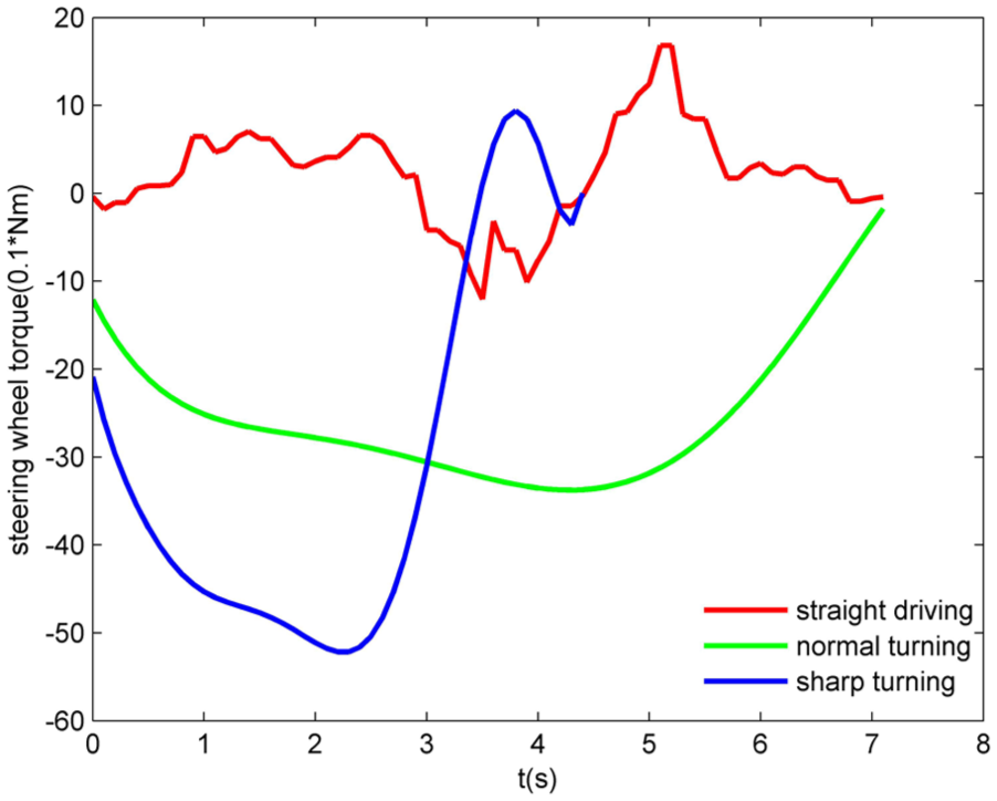
Steering wheel torque in normal turning, sharp turning and straight driving.

Therefore, principal component analysis (PCA) is used to select reasonable feature parameters. PCA can analyse multivariate parameters and simplify them to finite feature parameters. In this article, five parameters, such as the steering wheel angle, the steering wheel angle velocity, the steering wheel torque, the rate of change of the steering wheel torque and the angle acceleration of the steering wheel, are alternative feature parameters. PCA is used to calculate the contribution rates of these features. In the process of PCA, parameters with higher contribution rates represent larger amounts of the information in the original data.

The PCA results of five alternative feature parameters are shown in Table 1. Parameters 1–5 are the steering wheel angle, the steering wheel angle velocity, the steering wheel torque, the rate of change of the steering wheel torque, and the angle acceleration of the steering wheel. From the first parameter to the fifth parameter, the parameter variance and contribution rate decrease successively; thus, the amount of information contained in each parameter gradually decreases. The cumulative variance contribution rate of the first two parameters is 70.624%. However, the cumulative variance contribution rate of the first three parameters is 86.586%, which is greater than that of the first two parameters. To avoid the loss of key information, the retained parameter cumulative variance contribution rate should generally exceed 85%. Therefore, the first three parameters contain almost all of the information. Considering the above factors, this study employs the steering wheel angle, the steering wheel angle velocity and the steering wheel torque as feature parameters for use in driver steering intention identification.

Table 1.

PCA analysis results.

Parameter	Variance	Contribution rate (%)	Cumulative contribution (%)
1	1.971	39.492	39.492
2	1.560	31.132	70.624
3	0.798	15.962	86.586
4	0.510	10.193	96.778
5	0.161	3.222	100.000

PCA: principal component analysis.

The establishment of the GHMM

Driver actions are external expression to the perception of current driving environment and the concrete manifestation of drive intention. ¹⁷ The turning operation is a complex event and last for a certain period of time. Therefore, driver behaviour should be recognized from turning actions over a period of time, instead of a single state.

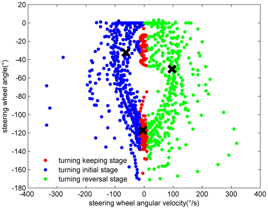
Analysis of the experimental data shows that the turning process can be divided into the turning initial stage, the turning keeping stage and the turning reversal stage, as shown in Figure 3. Normally, turning intention is recognized in the second stage of the turning process, the turning keeping stage, which is a relatively stable state. However, as shown in Figure 3, at the end of the turning keeping stage, more than half of the whole turning process has been completed. If turning intention is recognized in this stage, the vehicle stability control and steer-by-wire strategies based on driver intention will cause system delays. Driving safety will thus be affected, especially in the sharp turning. To improve turning safety and the real-time performance of driver turning intention recognition, the initial turning stage is chosen to recognize the turning intention.

Figure 3.

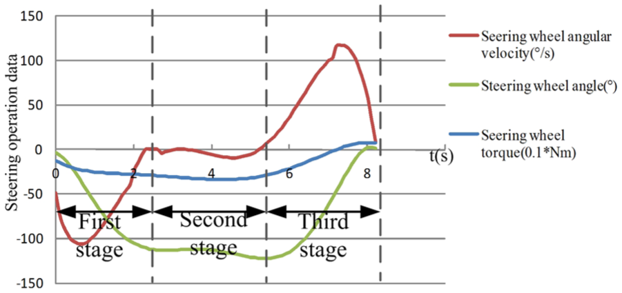
Steering wheel operation process.

The particular order of the short-term behaviour reflects driver intentions produced under current driving conditions. HMM can recognize driver intention by observing driver behaviour ordering.^7,8 The state of the observation matrix sequence is represented by the output probability of the Gaussian mixture model in the GHMM. The recognition accuracy of the GHMM can be improved by increasing the number of Gaussian mixtures. ⁶

Based on the turning initial stage, sharp turning and normal turning GHMMs are established separately. The observation sequence of the GHMM can be described as a multi-dimensional vector

$$O_t=\{a\left(t\right),b\left(t\right),c\left(t\right)\}$$

(1)

where $a(t)$ is the steering wheel angle, $b(t)$ is the steering wheel torque and $c(t)$ is the steering wheel angular velocity.

The Baum–Welch algorithm is used to optimize the three parameters of the GHMM, which are described as $\lambda =(\pi ,A,B)$ , where $\pi$ is the initial state distribution, A is the state transition probability matrix and B is a probability density function.

The probability density function of the model is

$$b_i\left(O\right)=\sum _{j=1}^M{\omega }_{\mathrm{ij}}N(O,{\mu }_{\mathrm{ij}},{\sigma }_{\mathrm{ij}})$$

(2)

where $N(O,{\mu }_{\mathrm{ij}},{\sigma }_{\mathrm{ij}})$ is the j-dimensional Gaussian probability density of state i, O is the observation sequence, ${\mu }_{\mathrm{ij}}$ is the mean of the Gaussian function and ${\sigma }_{\mathrm{ij}}$ is the covariance of the Gaussian function.

Assuming that ${\epsilon }_t(i,j)$ is the probability of the jth Gaussian mixture function in the state observation sequence i at time t, the probability that the Markov chain is in state j at time $t+1$ is as follows

$$\begin{array}{c}{\epsilon }_t(i,j)=\frac{p(s_t=i,s_{t+1}=j,O|\lambda )}{p(O|\lambda )}\hfill \\ =\frac{{\alpha }_t(i){\beta }_t(i)}{\sum {\alpha }_t(i){\beta }_t(i)}\times \frac{{\omega }_{\mathrm{ij}}P[O,{\mu }_{\mathrm{ij}},\sigma ]}{\sum _1^K{\omega }_{\mathrm{ij}}P[O,{\mu }_{\mathrm{ij}},\sigma ]}\hfill \end{array}$$

(3)

where ${\mu }_{\mathrm{ij}}$ is the mean matrix of the Gaussian mixture function, $\sigma$ is the mixed covariance matrix and ${\omega }_{\mathrm{ij}}$ is the weight of output probabilities of different Gaussian mixture functions. Based on the Gaussian mixture model, the parameter re-estimation is as follows

$$\omega {\prime }_{\mathrm{ij}}=\frac{\sum _{t=1}^T{\epsilon }_t(i,j)}{\sum _{t=1}^T\sum _{t=1}^K{\epsilon }_t(i,j)}$$

(4)

$$\mu {\prime }_{\mathrm{ij}}=\frac{\sum _{t=1}^T{\epsilon }_t(i,j)O_t}{\sum _{t=1}^T{\epsilon }_t(i,j)}$$

(5)

$$\sigma {\prime }_{\mathrm{ij}}=\frac{\sum _{t=1}^T{\epsilon }_t(i,j)(O_t-{\mu }_{\mathrm{ij}}){(O_t-{\mu }_{\mathrm{ij}})}^{\prime }}{\sum _{t=1}^T{\epsilon }_t(i,j)}$$

(6)

After the optimization of the parameters of the GHMM, the matching between the collected data and GHMM is calculated using the forward–backward algorithm. The training process of the GHMM is shown in Figure 4.

Figure 4.

Training process of the GHMM.

The establishment of the GGAP-RBF neural network

To improve the classification ability of the model, function (7) is no longer used to recognize turning intention. Instead, turning intention is described as a function of the log-likelihood of the two GHMMs given test data ( $\mathrm{loglik}1$ and $\mathrm{loglik}2$ ), the vehicle yaw rate ${\omega }_r$ and the lateral acceleration $a_y$ shown in function (8). However, a precise mathematical model is difficult to formulate because of the strong nonlinear characteristics of the system

$$\mathrm{Intention}=max(\mathrm{loglik}1,\mathrm{loglik}2)$$

(7)

$$\mathrm{Intention}=F(\mathrm{loglik}1,\mathrm{loglik}2,{\omega }_r,a_y)$$

(8)

Neural network can be used to solve the problem described above because they have strong nonlinear mapping ability, self-learning ability and good adaptability. In this article, a RBF neural network is adopted to establish the upper layer of the driver turning intention recognition model. As turning operation times and neural network training times increase, the size and complexity of the network also increase, leading to the appearance of redundant neurons. Hence, resource allocation network (RAN) and pruning algorithm are used to optimize the growth of neurons. These algorithms can remove insignificant neurons and simplify the structures of neural network with large amounts of data. This type of model is called a GGAP-RBF neural network.^18–21

As shown in Figure 5, the RBF consists of an input layer, a hidden layer and an output layer. The Gaussian function is used as the transfer function of the neurons to realize the nonlinear mapping from the input layer to the hidden layer.

Figure 5.

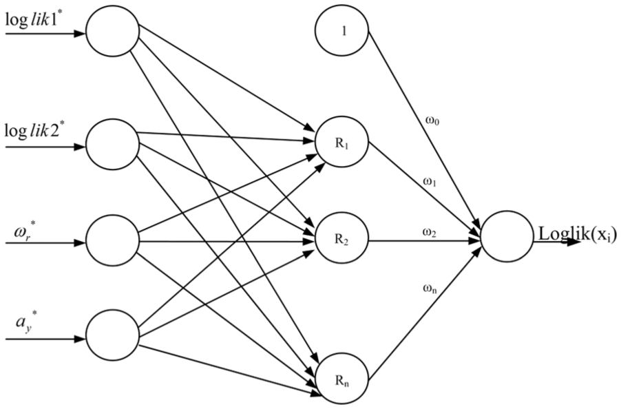
Topology and architecture of RBF neural network.

In the input layer, the input parameter is a vector of the log-likelihood of the two GHMMs and the yaw rate and lateral acceleration of the vehicle, which have already been normalized by the standard deviation, as shown in equation (9). The output of the layer is the driver turning intention

$$x_i=[\mathrm{loglik}{1}^{*},\mathrm{loglik}{2}^{*},{{\omega }_r}^{*},{a_y}^{*}]$$

(9)

$$f\left(x_i\right)=\mathrm{loglik}(x_i)={\omega }_0+\sum _{k=1}^K{\omega }_k·e^{-(\parallel w_k-x_i{\parallel }^2/{\sigma }_k^2)}$$

(10)

where $\mathrm{loglik}{1}^{*}$ , loglik 2^*, ${\omega }_r^{*}$ and $a_y^{*}$ represent the deviation standardization of $\mathrm{loglik}1$ , $\mathrm{loglik}2$ , ${\omega }_r$ and $a_y$ ; ${\omega }_k$ is the centre of the RBF of the kth neuron and ${\sigma }_k$ is the standard deviation of the Gaussian function, which indicates the width of the Gaussian function.

After the ith training iteration, RAN is used to optimize the growth of neurons. If a new neuron is added, the neuron parameters are given in equation (11)

$$\{\begin{array}{c}{\omega }_n=e_i\hfill \\ \multicolumn{1}{c}{w_n=x_i}\\ \multicolumn{1}{c}{{\sigma }_n=\kappa \Vert x_i-w_{\mathrm{ir}}\Vert }\end{array}$$

(11)

where ${\omega }_n$ is the weight connecting the new neuron to the output neuron, $w_n$ is the centre of the new neuron, ${\sigma }_n$ is the width of the new neuron, $e_i=y_i-f^{(i-1)}(x)$ is the error of the a priori estimate, $\kappa$ is an overlap factor that determines the overlap of the responses of the hidden neurons in the input space and $w_{\mathrm{ir}}$ is the centre value of the hidden neuron nearest to $x_i$ .

The worth of the new neuron is estimated using equation (12). If the condition is met, the new training data are valuable to the network, and the network performance is improved effectively by the new neuron. As a result, the new neuron is added, and the training data are accepted. If not, the training data and the new neuron are rejected

$$\{\begin{array}{c}\Vert x_i-w_{\mathrm{ir}}\Vert >{\epsilon }_i\hfill \\ \multicolumn{1}{c}{e_i=y_i-f(x_i)>e_{min}}\end{array}$$

(12)

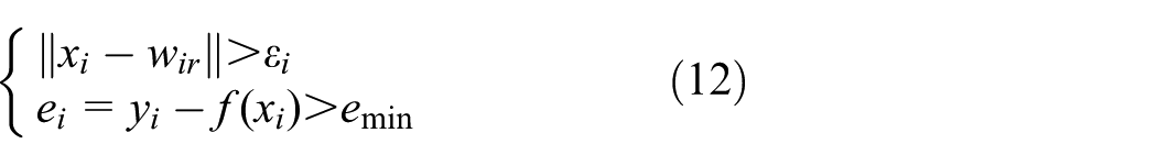
where ${\epsilon }_i$ and $e_{min}$ are the threshold of the distance and the error, respectively; $w_{\mathrm{ir}}$ is the centre value of the hidden neuron nearest to $x_i$ and $e_i$ is the error of the priori estimate.

And then, insignificant neuron should be judged and removed using pruning algorithm. The mean squared error of prediction output after the kth neuron is removed from the network in the ith training iteration is as follows

$$\begin{array}{c}{\mathrm{E}}_q\left(k\right)=\Vert \epsilon (k,1),\epsilon (k,1),\dots ,\epsilon (k,n){\Vert }_{\mathrm{q}}\hfill \\ ={\left(\frac{1}{n}\sum _{i=1}^n{\epsilon }^q(k,i)\right)}^{\frac{1}{q}}=\Vert {\omega }_k{\Vert }_q{\left(\frac{1}{n}\sum _{i=1}^n{R}_k^q\left(x_i\right)\right)}^{\frac{1}{q}}\hfill \end{array}$$

(13)

where $R_k(x_i)$ is the Gaussian RBF, n is the training time, $\Vert {\Vert }_q$ is the q-norm of vectors and k is the kth hidden neuron.

The inputs of the RBF, $\mathrm{loglik}{1}^{*}$ , $\mathrm{loglik}{2}^{*}$ , ${\omega }_r^{*}$ and $a_y^{*}$ , follow the normal sampling distribution $N(\mu ,{\sigma }^2)$ independently. The sample range of the ith training data $(x_i,y_i)$ is X, which is divided into J small parts ${\mathrm{\Delta }}_j$ . Each part is equal

$${\mathrm{E}}_q\left(k\right)=\frac{1}{n}{\Vert {\omega }_k\Vert }_{\mathrm{q}}{\left({\displaystyle \sum _{j=1}^n{R}_k^q\left(x_j\right)n\frac{1}{\sqrt{2\pi }\sigma }\exp \left(-\frac{\left(x_j-\mu \right)}{2{\sigma }^2}\right)S\left({\mathrm{\Delta }}_j\right)}\right)}^{\frac{1}{q}}$$

(14)

As ${\mathrm{\Delta }}_j$ tends to infinity, the sum over the sample range becomes approximately equal to the integral value

$$\begin{array}{c}{E}_{\mathrm{sig}}\left(k\right)=\underset{j\to \infty }{lim}{E}_q\left(k\right)\hfill \\ =\Vert {\omega }_k{\Vert }_q\underset{I=1}{\overset{2}{\Pi }}{\left(\underset{a1}{\overset{b1}{\int }}{e}^{-({\Vert {\omega }_k-x_{i,\mathrm{I}}\Vert }^2/{\sigma }_k^2)}{P}_1\left(x\right)\mathrm{dx}\right)}^{\frac{1}{q}}\hfill \end{array}$$

(15)

where E_sig(k) is the significance of the kth neuron to the network, which means the contribution of that neuron to the whole network. $P_1(x)$ is the probability distribution function. If E_sig(k) is less than the learning accuracy e_min, the neuron is considered to be insignificant and is removed. Otherwise, the neuron is significant and should be retained. Insignificant neurons can be removed from the GGAP-RBF neural network; thus, the size of the network can be limited to a reasonable range. The training process of the GGAP-RBF neural network is shown in Figure 6.

Figure 6.

Training process of the GGAP-RBF neural network.

Modelling and statistical analysis

Experimental programme

The experiment was carried out at the comprehensive automobile performance testing ground of Chang’an University, which is shown in Figure 7. Due to the effects of vehicle speed and turning radius on driver intention, in order to ensure that the driver would display obvious sharp turning and normal turning intentions in the experiment, the vehicle speed and test road turning radius needed to be determined.

Figure 7.

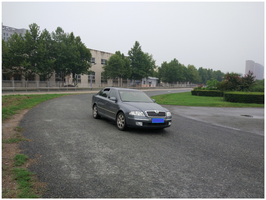
Automobile performance testing ground at Chang’an University.

According to the Specification for Design of Municipal Roads (CJJ37-2012) and the Specification for Design of Interactions on Urban Road (CJJ152-2010), the radius of curbs at intersections is required to be 10–30 m. Moreover, the snake cornering and double-lane change conditions in the Vehicle Handling Stability Test Method (GB/T6323-2014) are analysed. Given that the minimum turning radius of the test vehicle is 5.6 m, the radius of curvature of the test track was set to 10, 15, 20, 25, 30, 35, 40, 45 and 50 m preliminarily. In addition, speeds of 10, 20, 30, 40 and 50 km/h were used in the test. The radius of the turning test track and the speed are then specified in pairs as the initial test conditions. From the subjective expression of the experimenters, drivers will not generate sharp turning intentions at a speed of 10 km/h. When the vehicle speed exceeds 30 km/h with a turning radius of 10, 15, 20, 25 or 30 m, a driver will not generate a normal turning intention. When the vehicle speed is less than 30 km/h with a turning radius of 35, 40, 45 or 50 m, a driver will not generate a sharp turning intention. Therefore, to simplify the experiment and ensure that the driver would display an obvious turning intention, the radius of curvature of the test track was set to 15, 30 and 45 m. In addition, speeds of 20, 30 and 40 km/h were used in the tests. To distinguish between straight driving and turning, straight driving tests were also conducted at speeds of 20, 30 and 40 km/h.

All of the experiments were carried out in the same test environment. To eliminate interference from the external environment, there were no other vehicles, pedestrians, obstacles or external disturbances. The test route was marked in advance to ensure the correct identification of the test routes. Driving experience, gender and personality can affect driver decision making. To eliminate the effects of different operators on the test results, three drivers with different levels of driving experience were selected. The tests followed the procedures described in the following:

1. In the straight driving, the test vehicle ran freely on the test track, while the driver is forbidden to manipulate the steering wheel.

2. In the normal turning, the test vehicle was accelerated or braked to constant specified speed before a specified position, and the driver then made a normal turn.

3. In the sharp turning, the test vehicle was accelerated or braked to constant specified speed before a specified position, and the driver then made a sharp turn.

The distribution of the test data is shown in Table 2. These data can be divided into two parts; three-quarters of the test data are used for offline training of the model, whereas the remainder are used for online verification of the model.

Table 2.

The distribution of the test data.

	20 km/h	30 km/h	40 km/h
Sharp turning	65	65	50
Normal turning	70	70	54
Straight driving	30	21	21

Data acquisition and processing

Both the GHMM and GGAP-RBF algorithms are self-learning algorithms; thus, a large number of learning samples are required. The steering wheel angle, the steering wheel angle velocity, the steering wheel torque and the vehicle speed make up the observations that are provided to the lower layer of the GHMM/GGAP-RBF hybrid model. The observations provided to the upper layer include the yaw rate and lateral acceleration. In the experiment, the steering wheel torque, the steering wheel angle and the steering wheel angle velocity are collected using a steering wheel sensor produced by Kistler. A VB2SX vehicle GPS produced by Racelogic is used to collect the vehicle speed. A IMU04 three-axis gyroscope is used to measure the longitudinal acceleration, the lateral acceleration and the yaw rate of the vehicle. Options of available data update rate of Kistler MSW Sensors are 5, 10, 20 and 100 Hz, and the max data update rate of VGPS is 10 Hz and that of IMU04 is 50 Hz. In order to ensure the real-time synchronous acquisition of sensor signals, the DEWE-3010, 16-channel data acquisition instrument, is used to record the real-time data. And the data sample rate is set at 10 Hz. The instruments used in the experiments are shown in Figure 8, and the characteristics of these instruments are given in Table 3.

Figure 8.

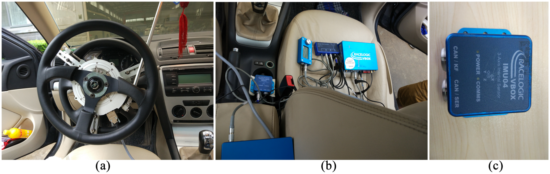
Instruments used in the experiments.

Table 3.

Characteristics of instruments.

Test equipment	Parameters measured	Range	Accuracy
Kistler MSW sensor	Steering torque	±250 N m	±0.15 N m
	Steering angle	±1250°	±0.1°
	Steering speed	±1000°/s
VBOX VGPS	Longitudinal speed	1609 km/h	0.01 km/h
IMU04	Longitudinal acceleration	±5g	± 0.15 mg
	Lateral acceleration	±5g	± 0.15 mg
	Yaw rate	±450°/s	± 0.001°/s

There are distinct differences between driver’s steering wheel operation, the brake pedal operation and the accelerator pedal operation. The driver only presses or releases the pedals when the driver intends to brake and accelerate, whereas the steering wheel is in the driver hands throughout the driving process. Therefore, the steering wheel will generate a certain torque and angle velocity all of the time. Hence, whether or not the steering wheel torque, the steering wheel angle and the steering wheel angle velocity are equal to 0 are not appropriate conditions for identifying driver turning operations. It is necessary to determine a threshold for driver turning intention. Therefore, the T-test is adopted to determine the threshold value of the steering torque, the steering angle and the steering wheel angle velocity for dividing experiment data into straight driving data and turning data. Because turning intention is identified in the turning initial stage in this article, the experimental data on the turning initial stage need to be extracted from the whole turning process. Therefore, the Gaussian mixture clustering method is used to extract the data on the turning initial stage from the sharp turning and normal turning for offline training of the GHMM. The data processing procedure is shown in Figure 9.

Figure 9.

Data processing procedure.

Hypothesis testing is a method for inferring general parameters from samples according to certain assumptions in mathematical statistics. The boundary thresholds of steering torque, steering angle and steering wheel angular velocity can be deduced using hypothesis testing. The T-test is adopted because the total standard deviation $\sigma$ is unknown. The boundaries determined by the T-test are shown in the following

$$x_{imax}=\overline{x}+\sigma \times T_p(n)=\overline{x}+\sigma \times \sqrt{\frac{n}{n-1}}{t}_p(n-2)$$

(16)

$$x_{imin}=\overline{x}-\sigma \times T_p(n)=\overline{x}-\sigma \times \sqrt{\frac{n}{n-1}}{t}_p(n-2)$$

(17)

where $\overline{x}$ is the sample mean value excluding $x_i$ , $\sigma$ is the sample standard deviation excluding $x_i$ , n is the sample size and $t_p(n-2)$ is the pth quantile of Student’s t-distribution with $n-2$ degrees of freedom. The much stricter two-sided test is chosen. In this test, $p=1-\alpha /2$ , $\alpha =0.01$ and $p=0.995$ .

The results of the T-test are shown in Figure 10. The boundaries of the steering wheel torque determined by the T-test are [0.02980, 2.38702]. The boundaries of the steering wheel angle are [−0.007, −0.0224], and those of the steering wheel angle velocity are [−9.5502, 9.9039].

Figure 10.

Straight driving boundaries determined by the T-test.

The data on the turning initial stage need to be extracted from the whole turning process for the turning intention is recognized in the turning initial stage. At the same time, the feature parameters differ significantly between the different turning intentions. Therefore, Gaussian mixture clustering methods are used to extract the data on the turning initial stage from the sharp turning and normal turning for GHMM model offline training. For normal turning, the steering wheel angle velocity–steering wheel angle clustering result is shown in Figure 11, and the steering wheel angular velocity–steering wheel torque clustering result is shown in Figure 12. Finally, training samples of normal turning GHMM are obtained.

Figure 11.

Clustering figure of steering wheel angular velocity–steering wheel angle for normal turning.

Figure 12.

Clustering figure of steering wheel angle velocity–steering wheel torque for normal turning.

For sharp turning, the steering wheel angular velocity–steering wheel angle clustering result is shown in Figure 13, and the steering wheel angular velocity–steering wheel torque clustering result is shown in Figure 14. Finally, samples for training the sharp turning GHMM are obtained.

Figure 13.

Clustering figure of steering wheel angle velocity–steering wheel angle for sharp turning.

Figure 14.

Clustering figure of steering wheel angle velocity–steering wheel torque for sharp turning.

Model training

A total of 280 groups of data on the turning initial stage are chosen for training the normal and sharp turning GHMMs offline. The parameters of the GHMM are shown as follows

$$\mathrm{GHMM}=\{\mathrm{prior},\mathrm{transmat},\mathrm{mix}\{N,\mathrm{mixmat},\mathrm{Sigma},\mathrm{mu}\}\}$$

(18)

where prior is the initial state matrix, transmat is the state transition matrix, mix is the Gaussian mixture parameter array, N is the number of Gaussian functions, mixmat is the weight of each Gaussian function in the GHMM, mu is the mean of each Gaussian function and Sigma is the covariance of each Gaussian function.

After the GHMM has been optimized many times, the parameters of the sharp turning GHMM are as follows

$$\begin{array}{c}N=3;\mathrm{prior}=\left[10\right]\hfill \\ \mathrm{transmat}=\left[\begin{array}{cc}0.9538\hfill & 0.0642\hfill \\ \multicolumn{1}{c}{0.0527}& 0.9473\hfill \end{array}\right]\hfill \\ \mathrm{mu}=[\mathrm{val}(:,:,1)\mathrm{val}(:,:,2)\mathrm{val}(:,:,3)]\hfill \\ \mathrm{val}(:,:,1)=\left[\begin{array}{c}\begin{array}{cc}-24.6391\hfill & -35.7854\hfill \end{array}\hfill \\ \multicolumn{1}{c}{\begin{array}{cc}-16.9701\hfill & -97.8132\hfill \end{array}}\\ \multicolumn{1}{c}{\begin{array}{cc}-77.4899\hfill & -35.1729\hfill \end{array}}\end{array}\right]\hfill \\ \mathrm{val}(:,:,2)=\left[\begin{array}{c}\begin{array}{cc}-34.5687\hfill & -40.7172\hfill \end{array}\hfill \\ \multicolumn{1}{c}{\begin{array}{cc}-63.2673\hfill & -40.9506\hfill \end{array}}\\ \multicolumn{1}{c}{\begin{array}{cc}-113.8177\hfill & -82.2767\hfill \end{array}}\end{array}\right]\hfill \\ \mathrm{val}(:,:,3)=\left[\begin{array}{c}\begin{array}{cc}-42.1960\hfill & -42.8578\hfill \end{array}\hfill \\ \multicolumn{1}{c}{\begin{array}{cc}-109.6440\hfill & -121.0544\hfill \end{array}}\\ \multicolumn{1}{c}{\begin{array}{cc}-34.1275\hfill & -10.2454\hfill \end{array}}\end{array}\right]\hfill \\ \mathrm{mixmat}=\left[\begin{array}{c}\begin{array}{ccc}0.2736\hfill & 0.3338\hfill & 0.3926\hfill \end{array}\hfill \\ \multicolumn{1}{c}{\begin{array}{ccc}0.1875\hfill & 0.0620\hfill & 0.7505\hfill \end{array}}\end{array}\right]\hfill \\ \mathrm{Sigma}=\left[\begin{array}{c}\mathrm{val}(:,1,1)\mathrm{val}(:,1,2)\mathrm{val}(:,1,3)\hfill \\ \multicolumn{1}{c}{\mathrm{val}(:,2,1)\mathrm{val}(:,2,2)\mathrm{val}(:,2,3)}\end{array}\right]\hfill \end{array}$$

The log-likelihood of the sharp turning and normal turning $\mathrm{loglik}{1}^{*}$ and $\mathrm{loglik}{2}^{*}$ , the vehicle yaw rate ${\omega }_r^{*}$ and the lateral acceleration $a_y^{*}$ , which have already been deviation standardization, are used to train the GGAP-RBF neural network. The parameters for the GGAP-RBF neural network are chosen as follows: ${\epsilon }_{max}=1.15$ , ${\epsilon }_{min}=0.04$ , $\gamma =0.999$ and $e_{min}={10}^{-4}$ . The growth of the hidden layer neurons during the offline learning process is shown in Figure 15. The number of hidden layer neurons is initially 0. As the number of training samples increases, the number of neurons of the GGAP-RBF also increases. A total of 11 insignificant neurons are found and removed in the training process. The same training samples are used to train the RBF model. The number of hidden neurons is 168, 11 more than the number of hidden neurons in the GGAP-RBF. Thus, GGAP-RBF can effectively reduce the size, computational cost and complexity of neural networks.

Figure 15.

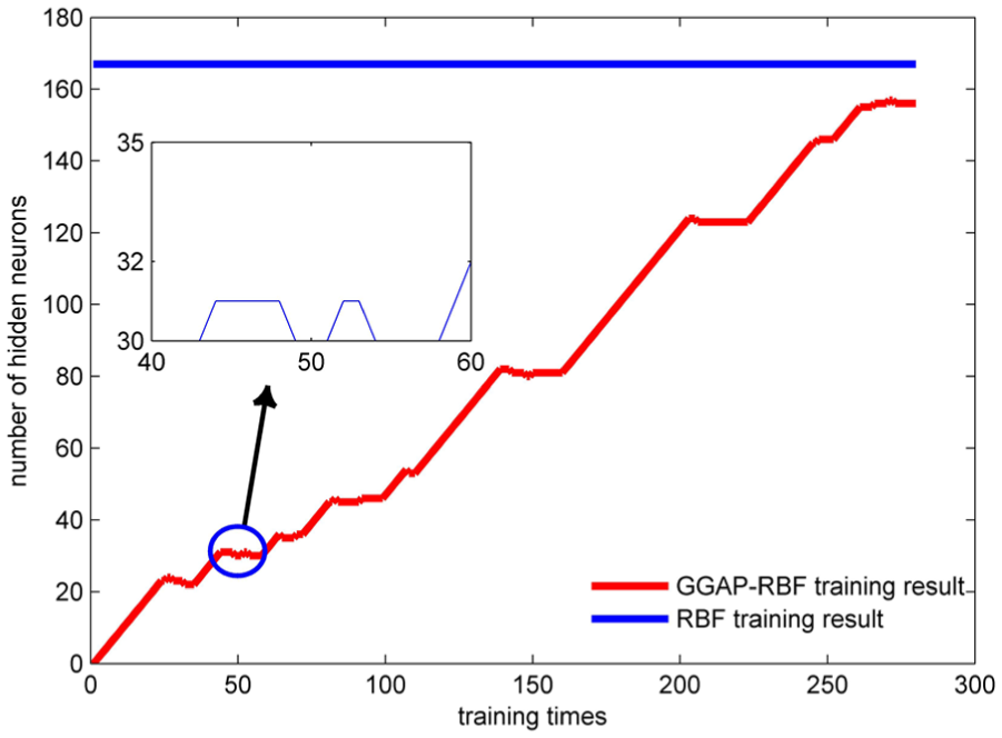
Numbers of hidden neurons in the GGAP-RBF and RBF.

Online recognition

Online recognition using the GHMMs

A total of 94 groups of data on the turning initial stage in normal and sharp turning condition are selected to make GHMM online recognition.

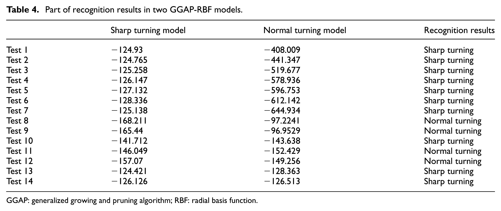
The accuracy of the two GHMMs is shown in Table 5. The results show that the recognition accuracy of the sharp turning GHMM is higher, and it reaches 100%. The recognition accuracy of the normal turning GHMM is only 72.34%. Part of recognition results in two GHMM models is shown in Table 4. Tests 1–7 involve sharp turning, whereas tests 8–14 involve normal turning. Table 4 shows that the log-likelihood of the two GHMMs under sharp turning conditions differs significantly. The difference between the two GHMMs reaches 226.59%. It is much easier to identify driver intention as sharp turning using function (7). However, under normal turning conditions (e.g. test 14), the log-likelihood of the sharp turning GHMM is −126.126 and that of the normal turning GHMM is −126.513. The difference between the two GHMMs is only 0.3068%. The differences are also very small in tests 10 and 13. Therefore, using only function (7) to recognize turning intention, all three of the normal turnings mentioned above are mistakenly identified as sharp turning. Thus, sharp turning intentions can be recognized correctly by the GHMMs, but mistakes may be made in identifying normal turning intentions.

Table 4.

Part of recognition results in two GGAP-RBF models.

	Sharp turning model	Normal turning model	Recognition results
Test 1	−124.93	−408.009	Sharp turning
Test 2	−124.765	−441.347	Sharp turning
Test 3	−125.258	−519.677	Sharp turning
Test 4	−126.147	−578.936	Sharp turning
Test 5	−127.132	−596.753	Sharp turning
Test 6	−128.336	−612.142	Sharp turning
Test 7	−125.138	−644.934	Sharp turning
Test 8	−168.211	−97.2241	Normal turning
Test 9	−165.44	−96.9529	Normal turning
Test 10	−141.712	−143.638	Sharp turning
Test 11	−146.049	−152.429	Normal turning
Test 12	−157.07	−149.256	Normal turning
Test 13	−124.421	−128.363	Sharp turning
Test 14	−126.126	−126.513	Sharp turning

GGAP: generalized growing and pruning algorithm; RBF: radial basis function.

Online recognition using the GHMM/GGAP-RBF hybrid model

SVM is one of the main methods used by researchers to recognize driver intention.^22–24 The SVM is also a self-learning pattern recognition method, and it displays relatively high learning accuracy and learning ability, even when based on limited sample information. A precise mathematical model is difficult to establish because of the strong nonlinear characteristics of the relationship between the steering wheel angle velocity, the steering wheel angle, the steering wheel torque and driver turning intention. Therefore, a nonlinear SVM is selected for comparison in studying the accuracy of the GHMM/GGAP-RBF hybrid model.

The same data from the turning initial stage used in the GHMMs are selected to enable online recognitions of GHMM/GGAP-RBF hybrid model and the SVM model. Some of the results are shown in Figure 16. Tests 1 to 4 represent sharp turnings, whereas tests 5 to 8 represent normal turnings. The identification results of the turning intention are expressed by −150 and −100, respectively.

Figure 16.

Identification results of the GHMM/GGAP-RBF hybrid model.

The accuracy of recognition obtained using the GHMM, the SVM model and the GHMM/GGAP-RBF hybrid model is shown in Table 5. The GHMM displays worse recognition effectiveness for the normal turning intention, for which the accuracy is only 72.34%. Table 5 shows that the GHMM/GGAP-RBF hybrid model yields the best precision, which can reach 100% for the sharp turning intention and 96.88% for the normal turning intention. The recognition method failed three times for the normal turning condition. The accuracy is 24.53% greater than that of with the GHMM, representing a clear increase. Moreover, the SVM-based model displays the worst precision. In particular, for the normal turning intention, the recognition accuracy of the SVM model is only 71%. It is mainly because the intention identification based on SVM recognizes the driver intention through the behaviour at a certain moment or the average and the variance value of the feature parameter in time period rather than behaviour that takes place over some period of time. Thus, the identification of turning intention using the SVM-based model obtains inadequate driver behaviour information and ignores the connection between preceding and following moments in time. Thus, its recognition accuracy is greatly reduced.

Table 5.

Accuracy of identification obtained using the three models.

Model	Sharp turning	Normal turning
GHMM	100%	72.34%
SVM	89%	71%
GHMM/GGAP-RBF	100%	96.88%

GHMM: Gaussian mixture hidden Markov model; GGAP: generalized growing and pruning algorithm; RBF: radial basis function; SVM: support vector machine.

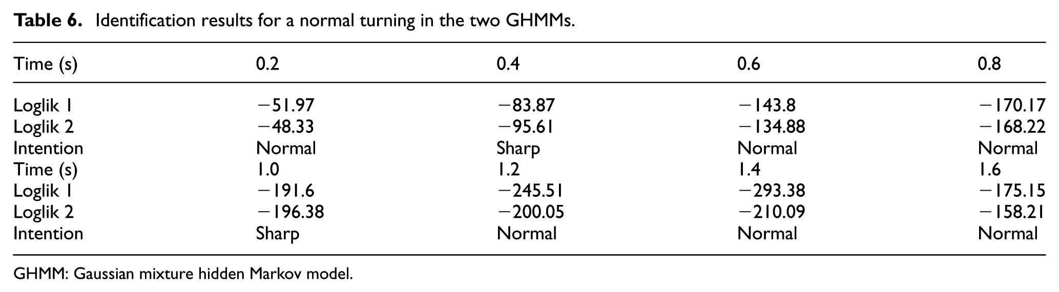
To further illustrate the classification ability of the GHMM/GGAP-RBF hybrid model, the process of identifying a normal turning using the GHMM and the GHMM/GGAP-RBF hybrid model is shown in Figure 17. The difference between the loglik values of the two models is very small, as shown in Table 6. Moreover, at 0.4 and 1 s, loglik 1 is greater than loglik 2, and the driver intention is incorrectly identified as a sharp turning. Although the GHMM reaches the correct conclusion at 0.2 and 0.8 s, given the minor difference, it is possible to obtain the opposite results from the same driver actions. Therefore, it can be inferred that this driver turning operation is on the boundary between a sharp turning and a normal turning. The actual driver turning intention is recognized accurately and in real time using the GHMM/GGAP-RBF hybrid model constructed in this study. Therefore, this model has contributed to solve the problem of overlapping classes.

Figure 17.

Identification process of the GHMM and hybrid models for a normal turning.

Table 6.

Identification results for a normal turning in the two GHMMs.

Time (s)	0.2	0.4	0.6	0.8
Loglik 1	−51.97	−83.87	−143.8	−170.17
Loglik 2	−48.33	−95.61	−134.88	−168.22
Intention	Normal	Sharp	Normal	Normal
Time (s)	1.0	1.2	1.4	1.6
Loglik 1	−191.6	−245.51	−293.38	−175.15
Loglik 2	−196.38	−200.05	−210.09	−158.21
Intention	Sharp	Normal	Normal	Normal

GHMM: Gaussian mixture hidden Markov model.

To discuss the robustness of the proposed framework to the full range of driver behaviours besides turning, the online identification of driver turning is carried out under the acceleration–turning and braking–turning condition.

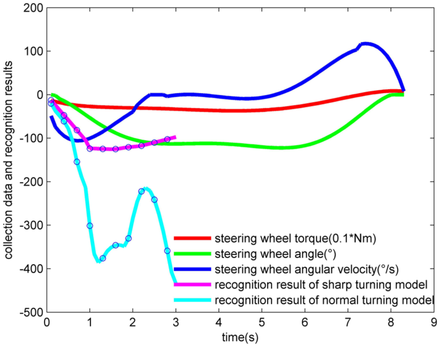
The acceleration–turning condition is shown in Figure 18. The vehicle is first driven in a straight line, and the acceleration is maintained. The vehicle speed is 40.688 km/h at 6.8 s. The driver then begins to make a normal turn, and the steering wheel reaches its original position at 12.6 s. Almost immediately, the driver begins to make a sharp turning. The identification process using the GHMM/GGAP-RBF hybrid model is shown in Figure 19. Using the boundary values of the steering wheel torque, the steering wheel angle and the steering wheel angle velocity inferred by the T-test, the driver intention is identified as straight driving from 0 to 6.8 s. At 6.8 s, the model determines that the driver starts the turning operation. Although the difference in the log-likelihood produced by the sharp turning and normal turning GHMMs is not obvious in the initial stage, the GHMM/GGAP-RBF hybrid model correctly identifies the driver intention as a normal turning. According to the results of Gaussian mixture clustering, at the end of the turning initial stage, the GHMM/GGAP-RBF hybrid model is no longer performing driver intention recognition. And this condition persists until the other turning process is identified. The normal turning ends after the turning reversal stage. The GHMM/GGAP-RBF hybrid model continues to identify the turning intention. The turning behaviour is identified as a sharp turning. Thus, it can be concluded that this model correctly identifies the driver turning intention under the acceleration–turning condition.

Figure 18.

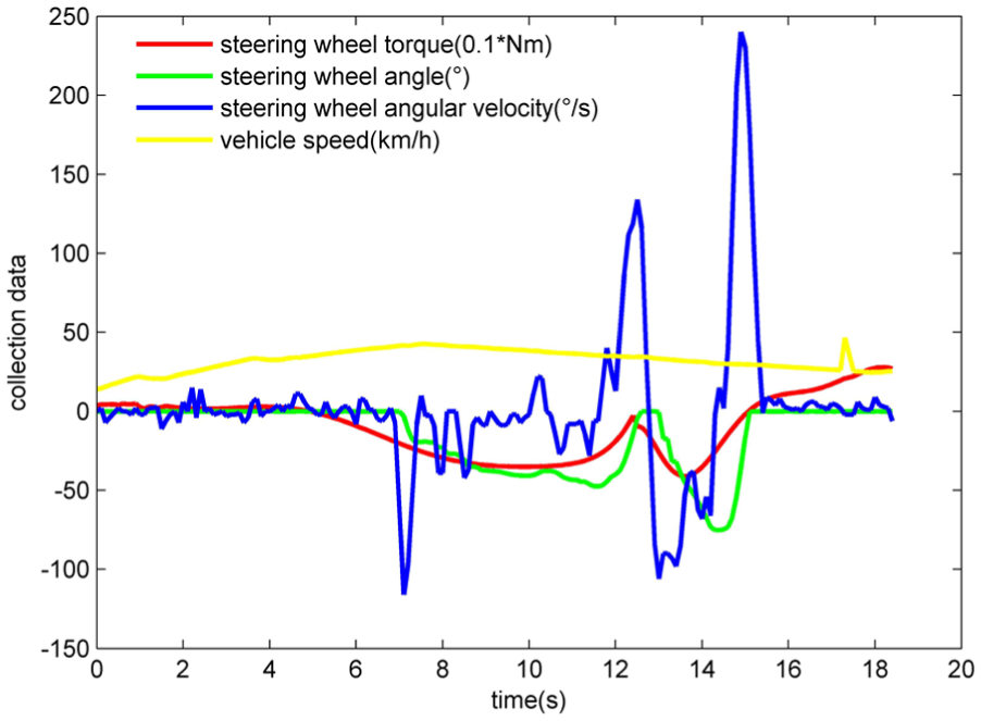
Acceleration–turning condition data.

Figure 19.

Identification process using the GHMM/GGAP-RBF hybrid model under acceleration–turning conditions.

The braking–turning condition is shown in Figure 20. The vehicle is first driven in a straight line and the braking is maintained. The vehicle speed is 32.873 km/h at 9.2 s. The driver then begins to make a sharp turn, and the steering wheel reaches its original position at 17.8 s. The identification process using the GHMM/GGAP-RBF hybrid model is shown in Figure 21. Using the boundary values of the steering wheel torque, the steering wheel angle and the steering wheel angle velocity inferred by the T-test, the driver intention is identified as straight driving from 0 to 9.2 s. At 9.2 s, the model recognizes that the driver starts the turning operation. Although at initial stage the log-likelihood difference between the sharp turning and normal turning GHMM is not obvious, the GHMM/GGAP-RBF hybrid model correctly identifies as the sharp turning intention. According to the results of Gaussian mixture clustering, at the end of the turning initial stage, GHMM/GGAP-RBF hybrid model is no longer performing driver intention recognition. And this condition persists until the other turning process is determined. Sharp turning ends after turning reversal stage. Thus, it can be concluded that this model correctly identifies the driver turning intention under the braking–steering condition.

Figure 20.

Braking–turning condition data.

Figure 21.

Identification process using the GHMM/GGAP-RBF hybrid model under braking–turning conditions.

Real-time analysis using the GHMM/GGAP-RBF hybrid model

The identification process using GHMM/GGAP-RBF hybrid model for a sharp steering is shown in Figure 22. Since the first stage of the turning, the turning initial stage, is chosen for the recognition of driver turning intention, the GHMM/GGAP-RBF hybrid model starts to work as soon as turning process is determined based on the results of Gaussian mixture clustering. The driver turning intention can be correctly recognize at 0.6 s. Based on the Gaussian mixture clustering method, the turning process enters turning keeping stage at 2.4 s. Therefore, using the existing HMM which is working in the turning keeping stage to recognize driver turning intention, the identification results will be obtained at least 2.4 s after the driver has begun to turn. This result is 1.8 s slower than the model used in this study. Therefore, the model proposed in this study displays substantial real-time performance.

Figure 22.

Identification process of the GHMM/GGAP-RBF hybrid model for a sharp turning.

To further illustrate the real-time performance of the GHMM/GGAP-RBF hybrid model, the elapsed time of getting the driver’s turning intention using the GHMM model and the GHMM/GGAP-RBF model is shown in Table 7. The time required by the GHMM/GGAP-RBF-based model is greater than that of the GHMM, mainly because the GHMM/GGAP-RBF model includes an upper layer (the GGAP-RBF model). The average additional elapsed time is 0.04949 s, the maximum additional time is 0.1331 s and the minimum additional time is 0.005 s. Therefore, it can be concluded that the elapsed time of the GHMM/GGAP-RBF model is not significantly greater than those of the GHMM.

Table 7.

Elapsed time of the GHMM and the GHMM/GGAP-RBF model.

Model	Test 1	Test 2	Test 3	Test 4
Hybrid model	0.578	0.6878	0.5903	0.4863
GHMM	0.5712	0.6488	0.5675	0.4562
Time difference	0.0068	0.039	0.0228	0.0698
Turning process	2.2	3.8	4.3	5.4
Model	Test 5	Test 6	Test 7	Test 8
Hybrid model	0.5576	0.536	0.715	0.4598
GHMM	0.4244	0.531	0.6732	0.4824
Time difference	0.1331	0.005	0.0418	0.0774
Turning process	4.0	3.5	3.2	1.8

GHMM: Gaussian mixture hidden Markov model; GGAP: generalized growing and pruning algorithm; RBF: radial basis function.

Table 7 also shows the elapsed time of a complete turning made by a driver. On average, the elapsed time of turning intention recognition is 17.985% of the time required for a complete driver turning process, and this proportion has a maximum value of 26.27%. Hence, the GHMM/GGAP-RBF hybrid model can quickly identify the correct turning intention after the driver begins to perform the turning operation.

Although slightly more time is required by the GHMM/GGAP-RBF hybrid model proposed in this study than the GHMM, it significantly improves the accuracy of driver turning intention identification. Therefore, the GHMM/GGAP-RBF model is more practical than the GHMM.

Conclusion

1. A GHMM/GGAP-RBF hybrid model is established to identify driver turning intentions based on experimental data and the analysis of steering wheel operation behaviours. GHMMs and GHMM/GGAP-RBF hybrid models are trained offline and made online recognition. And a nonlinear SVM is also selected for comparison. The results show that the recognition accuracy increases by 24.53%, reaching 96.88% for the normal turning and is 100% for the sharp turning. At the same time, the first stage of the turning, turning initial stage, is chosen for recognizing driver turning intentions. The new model is 1.8 s faster than the existing model. Compared with the GHMM and SVM, the identification accuracy and real-time performance of the hybrid model are significantly improved, especially in the normal turning. The goal of accurately identifying driving behaviour is realized.

2. In further studies, this model can be used to recognize acceleration intentions, braking intentions and complex working conditions, and it can also predict driver behaviour when combined with other algorithms. Applied to control systems, it will improve the safety and comfort of vehicle operation.