
Abstract
In order to meet the fine demand of different travelers, a multi-dimensional prediction method of travel time is proposed combining the toll collection data and meteorological data of highway. First, a logical model of multi-dimensional database is designed including vehicles’ dimension, meteorological dimension, and time dimension. Second, aiming at integration of the toll collection data and meteorological data, a matching method is presented within the space and time scale. Then, the multi-dimensional database is constructed. Next, an autoregressive moving average with exogenous input model is constructed using the travel time series and traffic flow series. The maximum likelihood estimation method is used to solve the parameters of the autoregressive moving average with exogenous input model. Considering the complexity and solving difficulty of the maximum likelihood equation, the particle swarm optimization algorithm is used to optimize the solution process. Finally, the toll collection data of two road links on Shenyang–Haikou expressway (G15) and the corresponding meteorological monitoring data are used to validate the algorithm. The results show that the prediction accuracy of the particle swarm optimization–autoregressive moving average with exogenous input model under normal and special conditions can be accepted and the absolute percentage error of road section between two neighboring toll stations is reduced by almost 5% after optimization.
Keywords
Introduction
Travel time prediction is an important part of intelligent transportation system (ITS). The prediction and publishing of travel time is significant to realize traffic flow guidance and improve road service quality. The travel time estimation and forecast studies are mainly based on the traffic data collected by loop vehicle detectors 1 and GPS. 2 However, in China, the highway is closed and there is a perfect network of toll system. The toll data are complete. The toll data record the types of vehicle, entry time, departure time, entry station, and departure station. This provides the possibility for travel time prediction. Some scholars have studied travel time prediction based on toll data. Faouzi and colleagues3,4 investigated the travel time estimation based on electronic toll collection (ETC) data alone by fusing them with other traffic data. Yoshikazu et al. 5 calculated travel time based on toll collection system data of Japan. Soriguera et al. 6 presented a new approach for measuring travel times based on closed toll highway data. Yamazaki et al. 7 used ETC data to calculate the average travel time and evaluate the network service level. Zhao et al.8,9 proposed a method of travel time prediction using highway toll data. At present, there are few studies on travel time prediction based on toll data, and all of them predict the average travel time of all vehicles on the road.
When traveling on a highway, the travel time of a vehicle is affected by a variety of weather (rain, snow, wind) factors. Regarding weather impact investigation on traffic operations, it is clear that weather conditions have a noticeable impact on traffic operations in various ways. Considering the impact of the weather on the traffic condition, Faouzi and Ben 3 designed a prediction algorithm that accounts for the weather impact during the prediction process. The result is considered accurate enough. Koesdwiady et al. 10 investigated the relevance of weather parameters and traffic flow based on deep learning networks and data fusion methods to improve the accuracy of traffic flow forecasts in bad weather. Qiao et al. 11 used traffic and weather data from multiple data sources to develop an integrated model that could predict travel times under various weather conditions. Qiu et al. 12 propose an integrated model for traffic flow parameter forecasting during inclement weather. Polson and Sokolov 13 used the deep learning architecture to forecast traffic flow, focusing on special weathers and events.
At the same time, there are different speed limits for cars and trucks on the highway, and the travel time of different vehicle models is different. Chen 14 analyzed the travel time data of highway, showing that there are significant differences in the travel time distribution between small passenger cars and buses. Zheng et al. 15 provided a model based on data fusion of multisource data to estimate travel times of different vehicle types on urban streets. Xia 16 analyzed the probability distribution of the travel time of different vehicle models and proposed that the probability distribution of expressway travel time is the mixed probability distribution model composed of the travel time of several vehicle models. Qian et al. 17 achieved multi-dimensional (time, space, vehicle model) traffic volume prediction based on highway toll data and the online analytical mining (OLAM) method. Bastard et al. 18 used the existing widespread inductive loop detector (ILD) network for realizing an estimation of individual travel time for a mixed population of cars and trucks.
However, most of the above literature only deals with the single impact of vehicle type or weather change on travel time prediction.
The research on travel time prediction started earlier and scholars have proposed many different algorithms. Innamaa 19 proposed a feedforward neural network prediction model of travel time, and the model was validated using the travel time data of the peak time interval on the weekend. On the basis of the above, Vanajakshi and Rilett 20 proposed the support vector machine (SVM) prediction model compared with the neural network model, and the results showed that the SVM model has better predicting precision. Zhao et al.8,9 proposed a method of travel time prediction using self-adaptive interpolation Kalman filter. Xu 21 applied the pattern matching method to establish the pattern library of travel time, and the K-nearest neighbor algorithm was used for library searching in order to predict travel time. Wu et al. 22 proposed a combination of K-means clustering and the autoregressive moving average with exogenous input (ARMAX) model method for travel time prediction, which was verified by vehicle detector data. Fei et al. 23 have developed a Bayesian inference-based dynamic linear model to robustly predict the exogenous factors (e.g. accidents), and they emphasize that the Bayesian approach enables the efficient update of travel time prediction contributing to online practicability. Some scholars pointed24–26 out that abrupt changes of traffic phenomena (e.g. lane changes, capacity drop, merge behavior, oscillations) can affect congestion development and propagation in various ways that require physical rather than statistical models to explain. The autoregressive and moving average (ARMA) model is a classic type of time series model for travel time prediction, with the inherent characteristics of time series for modeling and prediction, by which the random sequence can be predicted at high level of accuracy and following performance. The ARMAX model based on the ARMA model increases the regression variables to optimize prediction, improving the prediction problem of lagging. However, solving of the ARMAX is complex and difficult. Many studies are devoted to reduce the complexity and solving difficulty of ARMAX, in which some scholars use intelligent optimization algorithms to calculate the parameters of the ARMA model.27–29 In order to reduce the complexity and solving difficulty, this article introduces the particle swarm optimization (PSO) algorithm to optimize the solution process and use the optimized algorithm for travel time prediction.
In summary, it is very meaningful to make full use of the information provided by the toll data in China’s highway and to carry out the study of travel time prediction considering the impact of vehicle type or weather change. Moreover, the prediction results under different weather dimensions, vehicle type dimensions, and time dimensions are given. In this article, first, a multi-dimensional toll data warehouse is constructed based on the toll collection data and meteorological data. Second, the ARMAX model is established by setting traffic flow factors as the regression variables. Then, considering the complexity and solving difficulty, the PSO algorithm is used to optimize the solving process of model parameters. Finally, the travel time prediction under multi-dimensional factors can be achieved. The research content and framework of this article are shown in Figure 1.

Research content and structure.
Multi-dimensional database model
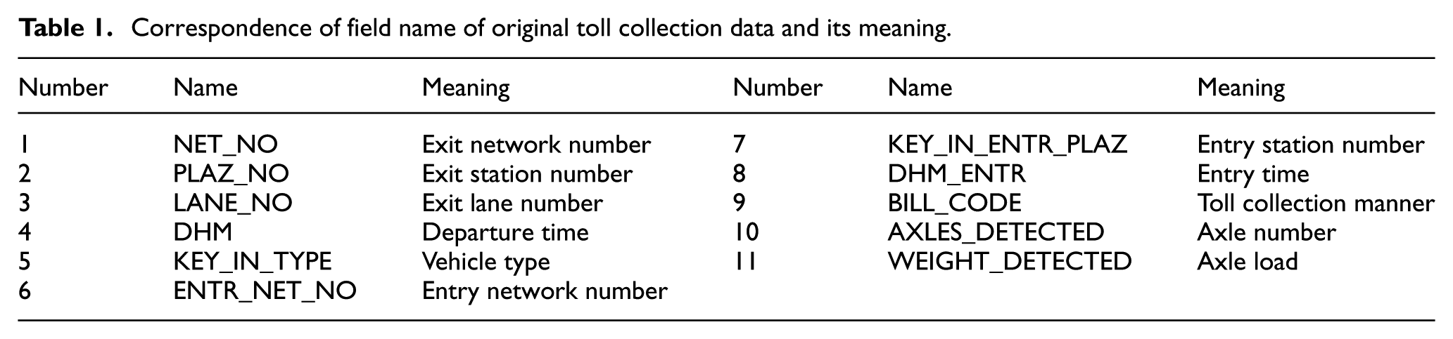
This study was carried out relying on the highway toll data and meteorological data. In the record of highway toll data, each line corresponds to the complete entry and exit information of a single vehicle. The information is described by 11 fields. The names and meanings of the fields are shown in Table 1.
Correspondence of field name of original toll collection data and its meaning.
The travel time can be obtained using the departure time minus the entry time, as shown in equation (1)

The meteorological data of the highway mainly record the types of weather, degree of weather (such as heavy snow, moderate snow, and light snow), start time, end time, route name, start location, end location, and so on.
Analysis of the influencing factors of travel time
This article studies the prediction of highway travel time, considering the impact of weather, vehicle type, period, and other factors. Therefore, the establishment of a complete highway toll database is the basis for completing the study. To build the database, first, we need to analyze the influencing factors of travel time.
Driving conditions are not the same under different weather, vehicle type, and period conditions on the same road section. Moreover, travel time will occur in varying degrees of fluctuations. The factors that affect the travel time between highway stations are summarized as follows:
Time. When the traffic flow exceeds the road capacity, traffic congestion will happen. There are a cyclical peak period and a low period of road traffic flow in 1 day. Similar changes are also present on different days of a week. Travel time changes in a regular manner with time.
Vehicle type. The driving characteristics will be different for different vehicle types in the same journey. The distributions of speed and traffic volume of different vehicle types also change over time. For instance, compared with trucks, the speed of small cars is faster and the travel time is relatively short under the same conditions; during the night, the proportion of trucks was significantly higher than that during the day.
Meteorological conditions. In the rain, snow, fog, and other meteorological conditions, highway traffic flow will be affected due to the reduced visibility, slippery road, and other reasons, resulting in the reduced driving speed or even congestion. Then travel time will increase.
The database model
The toll collection data record a large amount of commute information of single entrance–exit vehicles, including the entrance and exit gate names, the entrance and exit times, and the types of vehicles. In addition, the Highway Authority also generally records the meteorological monitoring data of road network, including rain, snow, fog weather types, starting and ending times, and starting and ending locations.
According to the analysis in the previous chapter, for the same link, the travel time varies in different degrees with different car type, time, and weather conditions. Based on these, a multi-dimensional database model is built. The period dimension, vehicle type dimension, and weather dimension were considered the three basic dimensions for the multi-dimensional database model. In addition, hierarchical dimensions were set up in each dimension. For instance, the period dimension includes the dimension of the day and the dimension of the week, the weather dimension includes rainy day dimensions, snow dimensions, and fog dimensions, and the vehicle type dimension includes the size dimension and the bus and truck dimensions. Figure 2 shows the basic structure of the multi-dimensional database model, where the leftmost side represents the fields of a complete database record and the right side represents the various dimensions of the multi-dimensional database model.
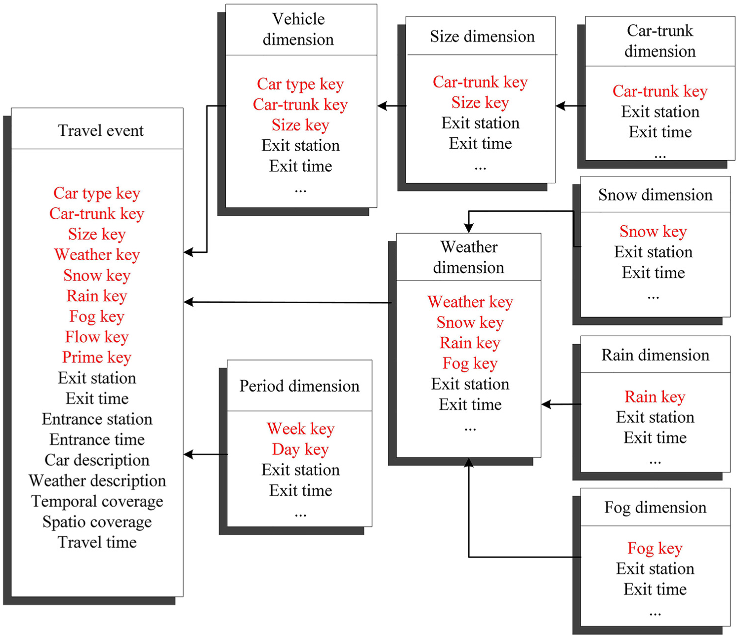
Model of the multi-dimensional data warehouse.
Data processing
Data transformation and data cleaning
There are many data with the problems of wrong form or abnormal value in the original data. Before the establishment of a complete highway traffic database, the wrong data should be removed according to the rules: 17 The entrance–exit times display abnormally, and the travel time is out of range obviously (more than 1 day) or the travel time is negative; data records are duplicate; there are the same entrance–exit time records.
The toll collection data with any characteristic mentioned above should be removed for data cleaning.
Data integration
The establishment of the multi-dimensional database model needs to match the toll data and meteorological data first. The mapping relationship between the weather and toll data can be established based on the core correlation parameters in the highway toll data and meteorological data. It specifically refers to the fields with the corresponding temporal and spatial meanings, including the vehicle entry time and the weather start time, the exit stake number of vehicle and the start stake number of weather, and so on.
Spatial matching
In the table of toll data, the vehicle’s inbound and outbound locations can be positioned by the KEY_IN_ENTR_PLAZ and PLAZ_NO fields. Moreover, in the table of weather data, the specific weather is positioned by the start location, the end location, and the route name fields. However, there is a limit that the weather data were only recorded in the same route. If a vehicle does not enter and leave on the same route, the meteorological conditions cannot be matched. Therefore, we only match and study the toll data records of vehicles that enter and leave the highway on the same route in this research.
Temporal match
In the table of toll data, the vehicle’s entry time and exit time can be positioned by the DHM_ENTR and ENTR fields. In the table of weather data, the specific time for which the weather occurs can be set by the start time and the end time field. Then the temporal match can be completed.
The influence degree of the meteorological factors
The matching rules of the toll collection data and the meteorological data are determined according to the influence degree of the meteorological factors influencing the travel route in the time and space scale, and the influence level is calculated as follows and marked in the database.
Assume that the initial influence level is 7, when the travel route is totally covered by the meteorological phenomenon in the time and space scale. Otherwise, after the determination of the space–time scale, the influence level may degrade; then, the final influence level is obtained and marked in the database as well. The process of obtaining the influence level is presented in Figure 3.
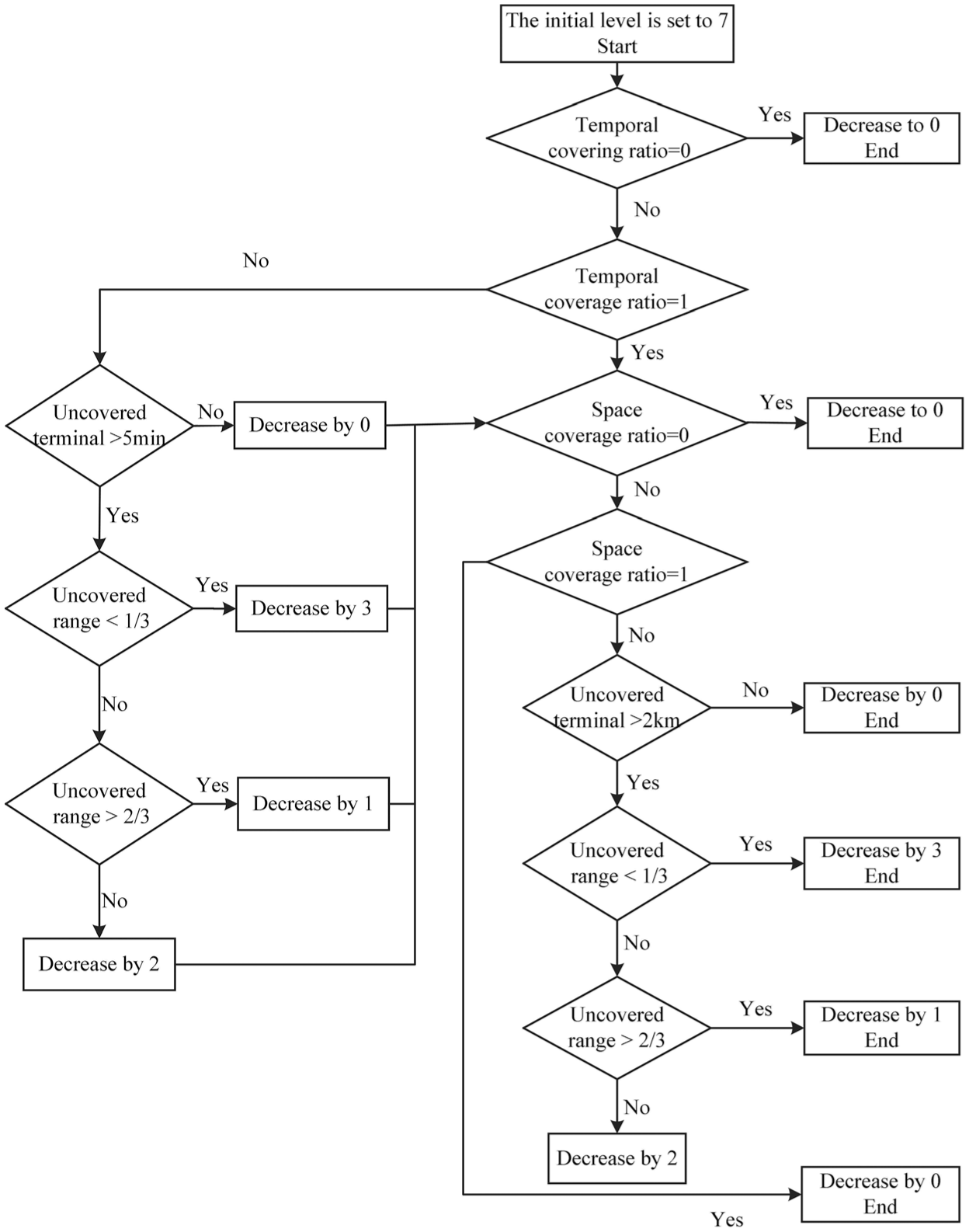
Data integration flow chart.
First, considering the influence level in the time scale, the initial influence level is 7, when the travel route is regarded as totally covered and the entrance time is within the 5-min interval of the meteorological starting time. The influence level will be 7. If the entrance time is out the 5-min interval of the meteorological starting time and the time scale coverage is more than 2/3, the influence degree will be declined by one level. Moreover, the influence degree will be declined by two levels, when the time scale coverage is less than 2/3 and more than 1/3. The influence degree will be declined by three levels when the time scale coverage is less than 1/3.
After the time scale determination, the space scale determination is required. The travel route is regarded as totally covered in the space scale when the entrance station is within 2 km of the meteorological starting point. If the entrance station is not within 2 km of the meteorological starting point, the influence degree will be discounted and decline. The influence degree will be discounted and declined by one level when the space scale coverage is more than 2/3. Moreover, the influence degree will be discounted and declined by two levels when the space scale coverage is less than 2/3 and more than 1/3. Moreover, the influence degree will be discounted and declined by three levels when the space scale coverage is less than 1/3.
After determination, there will be a value being uploaded to the database to represent the influence level of the meteorological factors.
Data filtering
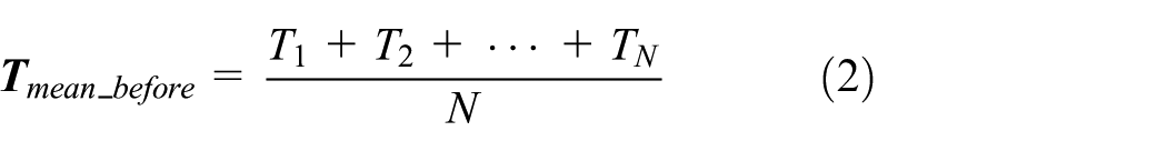
Based on the literature, 17 this article presents an improved quartile screening method. First, a relaxation coefficient is set for rough screening. Then the coefficient multiplication method is used to set the upper limit of the interval. Combined with the actual speed limit and mileage of the road link, the lower limit of the interval is set to complete the fine screening. The principle is shown as equations (2)–(8)


where
The original toll collection data of the Zhoushuizi–Jinzhou section on the Shenyang–Haikou expressway were used to verify the feasibility of the method. The outliers, that is, the travel time data noise, are removed using the improved quartile screening. The data of 320 cars were filtered out by coarse screening, 131 car data were filtered out by fine filter, 107 truck data were filtered out by coarse screening, and 131 car data were filtered out by fine filter. Taking the data of 1 day as the example, the travel time series of the target link is shown in Figure 4(a). Two distinct outliers are circled. The filtered travel time series obtained by the improved quartile method is shown in Figure 4(b). Two outliers are filtered. It can be seen that the data filtering method can remove the outlier effectively.

Travel time data processing: (a) before filtering and (b) after filtering.
Time series extraction
It is necessary to select a suitable time scale when obtaining the travel time series. The time periods of 10 and 15 min were set as the periods of cycle, respectively, and the time series were arranged in chronological order according to the entrance time. The travel time series of different time scales (10 and 15 min) are shown in Figure 5(a) and (b), respectively. Based on Figure 5(a) and (b), it can be seen that the 15-min period time series weakens the randomness of the data, truly reflects the variation characteristics of the travel time, and preserves the fluctuation characteristics. The 15-min period is enough to meet the actual prediction demand. Therefore, 15 min is selected as the time series cycle period in this article.

Time series of different time scales: (a) 10-min time series and (b) 15-min time series.
Travel time prediction principle
The ARMAX model

When a finite number of coefficients

which is named as the q-order moving average process, abbreviated as
The series themselves are used as the regression variables. Specifically, the p-order autoregressive process

If it is assumed that part of the series is autoregressive and the other part is moving average, a general time series model can be obtained as equation (12)

where the orders of the autoregressive moving average mixed process
The introduction of multiple correlation time series can help increase the fitting effect of the ARMA model and improve the prediction accuracy. The ARMAX model has the specific structure as follows

In equation (13),
Establishment of the ARMAX forecasting model
The basic idea of the ARMAX prediction model is as follows: first, the regression analysis of the relevant sequence and time series was done, obtaining the residuals and the linear relationship between the time series and its related series. Next, the ARMA model is used to model the residuals and then the short-time series is extracted as the model input. The prediction results of the two models are fused as the predicted results. This article extracts traffic flow series as the related series of the ARMAX model. The prediction flow chart is shown in Figure 6. This article mainly introduces the process of modeling the residual sequence using the ARMA model.

Prediction principle of the ARMAX model.
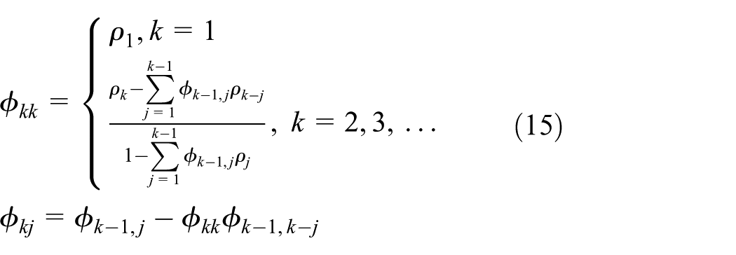
In general, the establishment of the ARMA model needs to go through the following steps: first, calculate the sample autocorrelation coefficient (ACF) values and the sample partial autocorrelation coefficient (PACF) values of the observed sequence. Second, perform model identification. According to the ACF and PACF values obtained in the previous step, the ARMA(p,q) model is fitted with the appropriate order. Third, estimate the value of the unknown parameter in the model. Fourth, verify the validity of the model. Finally, use the fitting model to predict the future trend of the sequence.
Model identification and parameter estimation
First, the sample ACF

The order of the model can be judged by the truncation characteristic of the ACF and the sample PACF.
In practice, because of the randomness of the sample, the correlation coefficient does not show the perfect situation of theoretical truncation. So a certain principle is needed to assist the order determination of the model. Quenouille proved that the sample ACF and the PACF obey the normal distribution

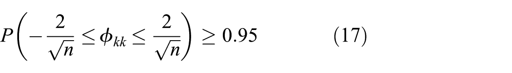
The two times range of standard deviation can be used for the judgment of truncation. If the ACF is significantly greater than the two times range of standard deviation, almost 95% of the ACF falls within the two times range of the standard deviation, and the process of decaying from a small non-zero ACF to a small value is very sudden, the ACF is usually regarded as truncated. The truncation order is d. If more than 5% of the sample correlation coefficient falls below the two times range of standard deviation, or if the process of decaying from a small non-zero ACF to a small value is relatively slow or very continuous, the correlation coefficient is not regarded as truncated.
The maximum likelihood estimation method is used to estimate the parameters. Under the maximum likelihood criterion, the likelihood function of the data sequence is given as follows

where
The partial derivatives of the unknown parameters

Make it equal to zero and simplify it

Since
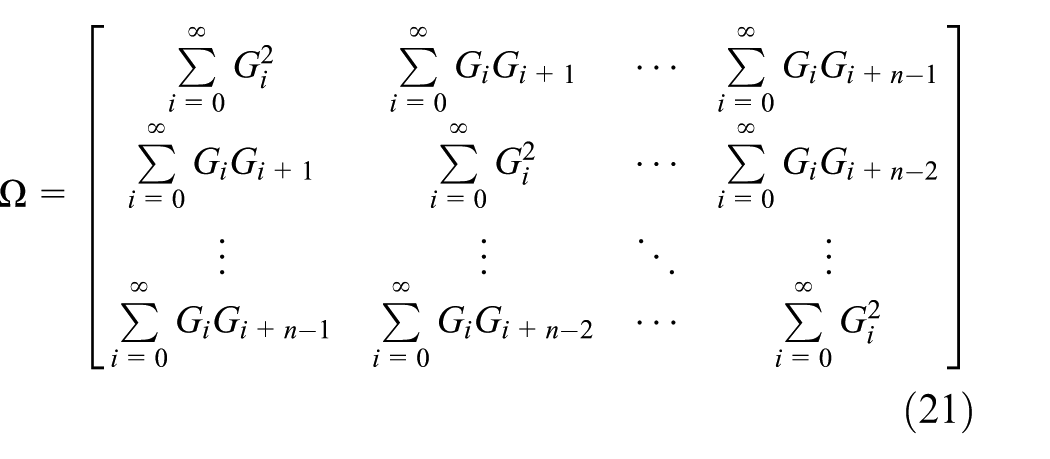
where
The PSO-ARMAX prediction model
Maximum likelihood estimation can take full advantage of the relationship between the sample sequences, but the transcendental equations under this model are complex. Moreover, the solution is very difficult and cannot be expressed by numerical solutions. Therefore, this article attempts to use the intelligent optimization algorithm in the model. The PSO algorithm is used to solve the maximum likelihood equation in the maximum likelihood estimation. Finally, the numerical solution of the model parameters is obtained.
The basic principle of PSO is as follows.
In the

where cl and c2 are the learning factors; ri1 and ri2 are the random numbers distributed uniformly on [0, 1]; and
The position of the k generation particle to the k + 1 generation particle is updated to

In order to make the objective function

where
Based on the above ideas, the solution space of the particle swarm is
The specific process of the algorithm proposed in this article is shown in Figure 6, where Gbest represents the global optimal position of each particle and Pbest represents the local optimal position of each particle.
Evaluation index of prediction error
According to the literature, 8 this article mainly uses the absolute percentage error and mean square error as the error evaluation indices of travel time prediction, which are calculated as follows
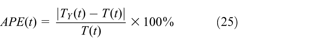


Here,
Test case of the prediction method
It is appropriate to extract 3–5 cycles of data of samples for model training. Therefore, the first five cycle periods of data were selected as the training samples of the prediction model and the training samples are updated with the update of the prediction moment. The short-term and real-time prediction of the travel time process can be obtained.
Road sections for experiment
Several sections of the Shenyang–Haikou expressway (G15) are adopted for the experiment. Toll stations on the experiment road are shown in Figure 7.

Toll stations on the experiment road.
Prediction results and error analysis
The travel time series of the Zhoushuizi–Jinzhou section and the Jinzhou–Sanshilipu section during 21 December 2014–21 January 2015 were extracted and used for rolling prediction, thus verifying the validity of the prediction model. First, the ARMA model was built. Then the associated traffic flow series were used as the regression variable to construct the ARMAX model. The evaluation of the prediction accuracy was carried out and the prediction effectiveness of the PSO-ARMAX model under different conditions was analyzed. In this article, the prediction results on 5 January 2015 are chosen, when there were snowy hours during the day, as the example to show more details.
Regression variable settings
Selecting 15 min as the cycle period of traffic flow series, the entrance traffic flows were counted and arranged as traffic flow series according to the entrance time. The cross-correlation analysis of the travel time and traffic flow is performed. The cross-correlation can be calculated using equation (29)
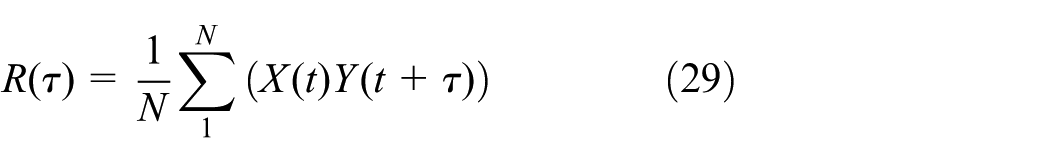
where
R software was used to analyze the cross-correlation between travel time and traffic flow series of cars and trucks, and the cross-correlation function graphs are plotted as shown in Figure 8(a) and (b). The two time series have a certain degree of correlation. In addition, the travel time series lag the flow series, which can be used as the regression variables to construct the ARMAX model.

Correlation of travel time series and traffic flow series: (a) correlation coefficient of cars and (b) correlation coefficient of trucks.
Results and error analysis
Take the Jinzhou–Sanshilipu section as the target. The prediction results of trucks using the ARMAX model and the PSO-ARMAX model are shown in Figure 9. The solid line represents the real travel time, the dashed line represents the predicted travel time using the ARMAX model, and the circular marker lines represent the predicted travel time using the PSO-ARMAX model. The prediction errors are shown in Figure 10.
The ARMAX and PSO-ARMAX model prediction results for the Jinzhou–Sanshilipu section on 5 January 2015.

Prediction error of the ARMAX and PSO-ARMAX models for the Jinzhou–Sanshilipu section on 5 January 2015.
The prediction process was carried out using the time series of a whole month. The prediction error of the whole month is shown in Table 2.
Prediction error evaluation for the Jinzhou–Sanshilipu section.

ARMAX: autoregressive moving average with exogenous input; PSO-ARMAX: particle swarm optimization–autoregressive moving average with exogenous input; MAPE: mean absolute percentage error; MSPE: mean square percentage error.
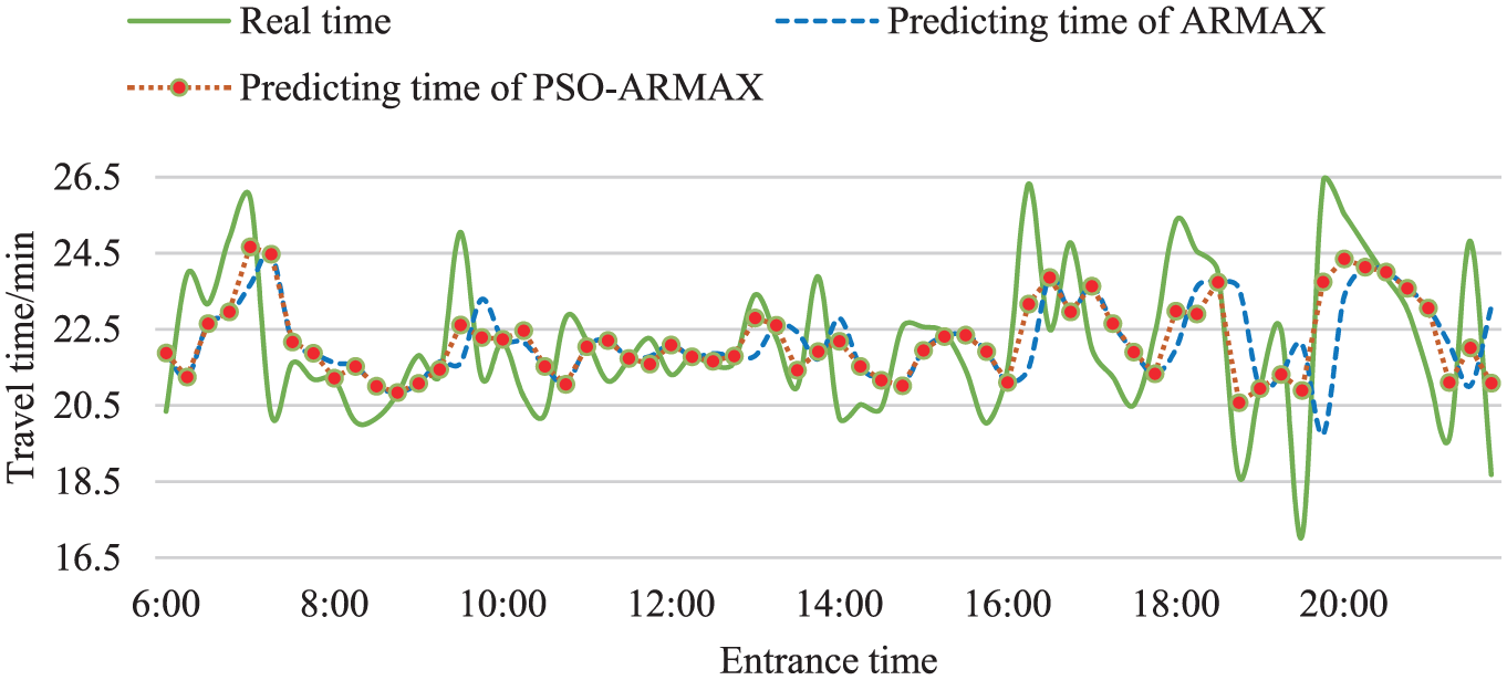
Take the Zhoushuizi–Jinzhou section as the target. The prediction results of trucks using the ARMAX model and the PSO-ARMAX model are shown in Figure 11. The solid line represents the real travel time, the dashed line represents the predicted travel time using the ARMAX model, and the circular marker lines represent the predicted travel time using the PSO-ARMAX model. The prediction errors are shown in Figure 12.

The ARMAX and PSO-ARMAX model prediction results for the Zhoushuizi–Jinzhou section on 5 January 2015.

Prediction error of the ARMAX and PSO-ARMAX models for the Zhoushuizi–Jinzhou section on 5 January 2015.
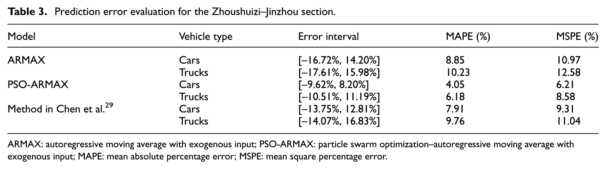
The prediction process was carried out using the time series of a whole month. The prediction errors of different vehicle types using the different models are shown in Table 3.
Prediction error evaluation for the Zhoushuizi–Jinzhou section.
ARMAX: autoregressive moving average with exogenous input; PSO-ARMAX: particle swarm optimization–autoregressive moving average with exogenous input; MAPE: mean absolute percentage error; MSPE: mean square percentage error.
It can be seen from the above table and figure that both the ARMAX and PSO-ARMAX models can give the acceptable prediction values. However, the PSO-ARMAX model can give better prediction results than the ARMAX model.
Then, we compared our method with that reported in Chen et al., 29 which uses intelligent optimization algorithms to calculate the parameters. The prediction results and errors are shown in Figures 13 and 14. The prediction error for a whole month is shown in Table 3. It can be seen that the prediction accuracy of the PSO-ARMAX method is higher than that of the method reported in Chen et al. 29

Prediction results of the PSO-ARMAX model and the method reported in Chen et al. 29 for the Zhoushuizi–Jinzhou section.
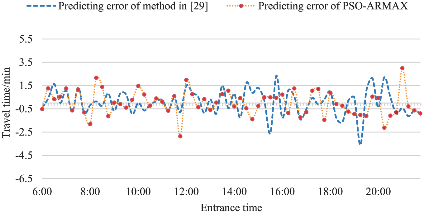
Prediction errors of the method reported in Chen et al. 29 and the PSO-ARMAX model for the Zhoushuizi–Jinzhou section.
Take the travel time forecast for 6:00–22:00 on 5 January 2015 as an example. According to the weather monitoring record, there was snow during 14:30–19:00. The prediction results of cars using the PSO-ARMAX model are shown in Figure 15. The prediction results of trucks using the PSO-ARMAX model are shown in Figure 16. The solid line represents the real travel time, the dashed line represents the predicted travel time of the PSO-ARMAX model. It can be seen that the PSO-ARMAX model can give good prediction results. In the case of cars, the travel time during the snow period has significantly increased, while the forecast model detected this trend and followed the real travel time. It can be inferred that the model can be applied in the accident or congestion conditions and achieve good predicting effect. For the trucks, the snow weather has little effect on the overall travel time, and the PSO-ARMAX prediction model gave acceptable predicting values.

Travel time prediction of cars for the Zhoushuizi–Jinzhou section.

Travel time prediction of trucks for the Zhoushuizi–Jinzhou section.
Error analysis and model comparison
It can be seen that the prediction accuracy of the cars is always higher than that of the trucks when comparing the prediction error of the travel time of cars with that of the trucks. The main reason is that the actual proportion of trucks in traffic is lower than that of cars. The toll collection data of trucks are less. Because of the scarcity of data, even if the interpolation is done, the sparseness of the data has not been fully improved, and the travel time data are highly fluctuating, which cannot fully reflect the real road condition and indirectly reduce the prediction effect of the model.
The results show that the PSO-ARMAX model is better than the ARMAX model. Mean absolute percentage error of the road section between two neighboring toll stations is reduced by almost 5%. The prediction accuracy is improved significantly. In this article, we focused on the travel time prediction of road sections, and the improvement effect is limited because of the short distance.
Conclusion
In this article, the prediction of highway travel time was studied using toll data. Some conclusions are as follows:
A multi-dimensional logic frame of database was constructed, and the integration method of the original toll collection data and the meteorological monitoring data was put forward; thus, a multi-dimensional data warehouse was built up.
This research used the ARMAX model for travel time prediction. The PSO algorithm was used to optimize the solving process of the model parameters, and setting the regression variables significantly reduces the mean absolute percentage error by almost 5%.
The application of travel time prediction in the examples shows that the PSO-ARMAX model has high accuracy in the prediction of travel time and can provide supporting evidences for traffic control and travel guidance. However, there is still much room for improvement in the prediction accuracy, and it can be achieved by improving the quality of the original data and adding the database dimension involving more factors, which have some influence on the travel time.
Through the above conclusions, here are some future research directions: this article carries out the prediction of travel time combining the highway toll data and the meteorological data. At present, the data fusion method is applied to the prediction research. In the future research, we can consider adding more data sources as well as events and accidents in order to enrich the multi-dimensional data warehouse and improve the prediction accuracy.
Footnotes
Handling Editor: Gang Chen
Declaration of conflicting interests
The author(s) declared no potential conflicts of interest with respect to the research, authorship, and/or publication of this article.
Funding
The author(s) disclosed receipt of the following financial support for the research, authorship, and/or publication of this article: This work was supported by “the Fundamental Research Funds for the Central Universities (2016JBM053).”