Sage Journals: Discover world-class research

Abstract

In today’s highly competitive global market, winning requires near-perfect quality. Although most mature organizations operate their processes at very low defects per million opportunities, customers expect completely defect-free products. Therefore, the prompt detection of rare quality events has become an issue of paramount importance and an opportunity for manufacturing companies to move quality standards forward. This article presents the learning process and pattern recognition strategy for a knowledge-based intelligent supervisory system, in which the main goal is the detection of rare quality events. Defect detection is formulated as a binary classification problem. The l₁-regularized logistic regression is used as the learning algorithm for the classification task and to select the features that contain the most relevant information about the quality of the process. The proposed strategy is supported by the novelty of a hybrid feature elimination algorithm and optimal classification threshold search algorithm. According to experimental results, 100% of defects can be detected effectively.

Keywords

Manufacturing classification threshold algorithm defect detection feature elimination algorithm model selection criterion quality control unbalanced data

Introduction

In today’s highly competitive global market, winning requires near-perfect quality, since intense competition has led organizations to low profit margins. Consequently, a warranty event could make the difference between profit and loss. Moreover, customers use Internet and social media tools (e.g. Google product review) to share their experiences, leaving organizations little flexibility to recover from their mistakes. A single bad customer experience can immediately affect companies’ reputations and customers’ loyalty.

In the quality domain, most mature organizations have merged business excellence, lean production, standards conformity, six sigma, design for six sigma, and other quality-oriented philosophies to create a more coherent approach.¹ Therefore, the manufacturing processes of these organizations only generate a few defects per million of opportunities. The detection of these rare quality events represents not only a research challenge but also an opportunity to move manufacturing quality forward.

Impressive progress has been made in recent years, driven by exponential increases in computer power, database technologies, machine learning (ML) algorithms, optimization methods, and big data.²

From the point of view of manufacturing, the ability to efficiently capture and analyze big data has the potential to enhance traditional quality and productivity systems. The primary goal behind the generation and analysis of big data in industrial applications is to achieve fault-free (defect-free) processes,^3,4 through intelligent supervisory control systems (ISCS).⁵

A learning process (LP) and pattern recognition (PR) strategy for a knowledge-based (KB) ISCS is presented, aimed at detecting rare quality events from manufacturing systems. The defect detection is formulated as a binary classification problem, in which thel₁-regularized logistic regression (LR) is used as the learning algorithm. The outcome of the proposal is a parsimonious predictive model that contains the most relevant features.

The proposed strategy is validated using data derived from two automotive manufacturing systems: (1) ultrasonic metal welding (UMW) battery tabs from a battery assembly process and (2) laser spot welding (LSW) sub-assembly components from an assembly process. The main objective is to detect low-quality welds (bad) from the processes.

The initial idea of rare quality event detection through KB ISCS was initially introduced in Escobar and Morales-Menendez.⁶ The proposal is extended—improved with respect to classification and parsimony—in this article with the introduction of two algorithms; these algorithms are aimed at addressing two of the most relevant challenges posed by the l₁-regularized LR algorithm. Challenges and theoretical properties are briefly discussed. To show the ability of the proposal in dealing with high-dimensional balanced data, another case study (LSW) is presented. Finally, to evaluate its performance, a comparative analysis is performed following a typical modeling analysis, and results are compared and briefly discussed.

The rest of this article is organized as follows: It starts with a review of the theoretical background in Section “LP and PR strategy” describes the proposal. Two studies in section “Case studies” followed by the “Comparative analysis.” Finally, “Conclusion” and “Future work” conclude this paper.

Theoretical background

The theoretical background of this research is briefly reviewed.

ML and PR

As discussed by Ghosh,⁷“As an intrinsic part of Artificial Intelligence (AI), ML refers to the software research area that enables algorithms to improve through self-learning from data without any human intervention.”ML algorithms learn information directly from data without assuming a predetermined equation or model. The two most basic assumptions underlying most ML analyses are that the examples are independent and identically distributed, according to an unknown probability distribution. PR is a scientific discipline that “deals with the automatic classification of a given object into one from a number of different categories (e.g. classes).”⁸

In ML and PR domains, generalization refers to the prediction ability of a learning algorithm model on unseen data.⁹ The generalization error is a function that measures well a trained algorithm generalizes.

In general, the PR problem can be widely broken down into three components: (1) feature space reduction, (2) classifier design and selection, and (3) classifier assessment.

Feature space reduction

In ML and PR, a feature is an individual measurable property of an observed phenomenon.¹⁰ The prediction ability of the classifier is determined by the inherent class information available in the features.¹¹ In general, a feature is good if its inherent class information is relevant to one of the class labels but is not redundant to other good features. If the correlation of two variables is used as a goodness measure, a good feature should be highly correlated to one of the class labels but not highly correlated to any other features.^12,13 A feature can be considered irrelevant if the information that it contains is independent from the class label.

The world of big data is changing dramatically, and feature access has grown from tens to thousands, a trend that presents enormous challenges in the feature selection (FS) context. Empirical evidence from FS literature exhibits that discarding irrelevant or redundant features improves generalization, helps in understanding the system, eases data collection, reduces running time requirements, and reduces the effect of dimensionality.^12–17 This problem representation highlights the importance of finding an optimal feature subset. This task can be accomplished by FS or regularization.

FS

Filter-type methods select variables independently of the classification algorithm or its error criteria, they assign weights to features individually and rank them based on their relevance to the class labels. A feature is considered good if its associated weight is greater than the user-specified threshold.¹² The advantages of feature ranking algorithms are that they do not over-fit the data and are computationally faster than wrappers, and hence, they can be efficiently applied to big datasets containing many features.¹³ However, most common methods—Mutual Information, ReliefF, and so on—do not help in removing redundant features, as features are evaluated independently; therefore, as long as features contain class discriminatory information, they will be selected, even if they are highly correlated to each other.^12,18,19

ReliefF is a well-known rank-based algorithm, and the basic idea for numerical features is to estimate the quality of each according to how well their values distinguish between instances of the same and different class labels. ReliefF searches for a $k$ of its nearest neighbors from the same class, called nearest hits, and also $k$ nearest neighbors from each of the different classes, called nearest misses; this procedure is repeated $m$ times, which is the number of randomly selected instances. Thus, features are weighted and ranked by the average of the distances (Manhattan distance) of all hits and all misses²⁰ to select the most important features,¹⁸ developing a significant threshold $τ$ . Features with an estimated weight below $τ$ are considered irrelevant and, therefore, eliminated. The proposed limits for $τ$ are $0 < τ \leq 1 / \sqrt{α m}$ ,²⁰ where $α$ is the probability of accepting an irrelevant feature as relevant.

Regularization

Another approach for FS is l₁ regularization. This method trims the hypothesis space by constraining the magnitudes of the parameters.²¹ Regularization adds a penalty term to the least square function to prevent over-fitting.²² The formulations of l₁ norm have the advantage of generating very sparse solutions while maintaining accuracy. The classifier-fitted parameters $θ_{i}$ are multiplied by a coefficient $λ$ to shrink them toward zero. This procedure effectively reduces the feature space and protects against over-fitting. Regularization methods may perform better than FS methods.²³

Classifier design, selection, and assessment

A classifier is a supervised learning algorithm that analyzes the training data (e.g. data with classification class) and fits a model. The training dataset is used to train a set of candidate models using different tuning parameters.

It is important to choose an appropriate validation or cross-validation (CV) method to evaluate the generalization ability of each candidate model and select the best, according to a relevant model selection criterion.

For information-theoretic model selection approaches in the analysis of empirical data, refer to Peruggia.²⁴ Common performance metrics for model selection based on recognition rates—correct decisions made—can be found in Fawcett.²⁵

For a data-rich analysis, the hold-out validation method is recommended, an approach in which a dataset is randomly divided into three subsets: training, validation, and testing. As an heuristic, 50% of the initial dataset is allocated to training, 25% to validation, and 25% to testing.²⁶

Once the best candidate model has been selected, it is recommended that the model’s generalization performance be tested on a new dataset before the model is deployed. This can also determine whether the model satisfies the learning requirement.²⁶ The generalization performance can be efficiently evaluated using a confusion matrix (CM).

CM

In predictive analytics, a CM²⁵ is a table with two rows and two columns that reports the number of false positives (FPs), false negatives (FNs), true positives (TPs), and true negatives (TNs). This allows more detailed analysis than just the proportion of correct guesses since it is sensitive to the recognition rate by class.

A type I error ( $α$ ) may be compared with a FP prediction; a type II ( $β$ ) error may be compared with a false FN.²⁷ They are estimated by

α = \frac{FP}{FP + TN}

(1)

β = \frac{FN}{FN + TP}

(2)

LR

LR, which uses a transformation of the values of a linear function, is widely used in classification problems. It is an unconstrained convex problem with a continuous differentiable objective function that can be solved either by the Newton’s method or the conjugate gradient. LR models the probability distribution of the class label $y$ , given a feature vector $x$ ²⁸

P (y = 1 | x; θ) = σ (θ^{T} x) = \frac{1}{1 + \exp (- θ^{T} x)}

(3)

where $θ \in R^{N}$ are the parameters of the LR model and $σ (\cdot)$ is the sigmoid function (logistic function) that maps values from $(- \infty, \infty)$ to $[0, 1]$ . The discrimination function itself is not linear, but the decision boundary is still linear.

The most common approach to estimate the parameters of a statistical model is to compute the maximum likelihood estimate (MLE). The problem of finding the MLE of the parameters θ for the unregularized LR can be defined by in terms of the negative log-likelihood (NLL)

min_{θ} \sum_{i = 1}^{M} - \log p (y^{(i)} | x^{(i)}; θ)

(4)

The NLL for LR is

NLL = - \sum_{i = 1}^{M} [y^{(i)} \log μ^{(i)} + (1 - y^{(i)}) \log (1 - μ^{(i)})]

(5)

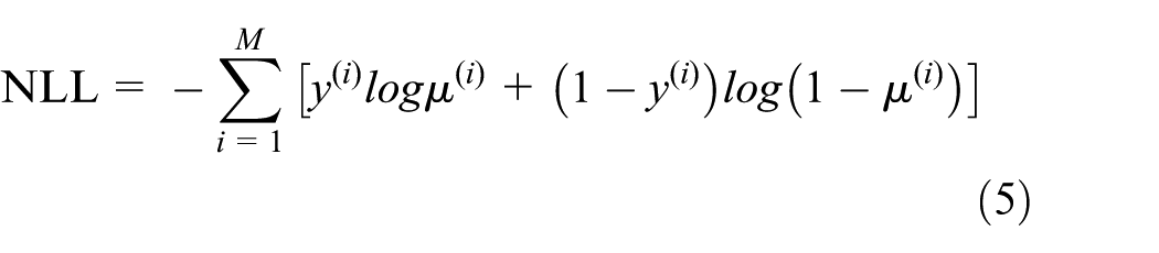
where $μ^{(i)} = sigm (θ^{T} x^{(i)})$ . It is also called the cross-entropy error (CEE) function.²⁹

Under the Laplacian prior $p (θ) = (λ / 2)^{N} \exp (- λ | | θ | |_{1}) (λ > 0)$ , the maximum a posteriori (MAP) estimate of the parameters $θ$ is

min_{θ} \sum_{i = 1}^{M} - \log p (y^{(i)} | x^{(i)}; θ) + λ | | θ | |_{1}

(6)

This optimization problem is referred to as l₁-regularized LR. This algorithm is widely applied in problems with small training sets or with high-dimensional input space. However, adding the l₁ regularization makes the optimization problem computationally more expensive. For solving the l₁-regularized LR,³⁰ the least absolute shrinkage and selection operator (LASSO) is an efficient method.

As the value of $λ$ increases, the number of features included in the model decreases. The higher the value of $λ$ , the lower the chance of over-fitting with too many redundant or irrelevant variables. The value of $λ$ can be tuned through validation or CV.

In general, high correlations among features may hamper the LASSO in finding the true model. LASSO may not be able to distinguish true features with any amount of data and any amount of regularization.³¹ Therefore, eliminating highly correlated features is one of the main challenges.

ISCS

ISCSs are computer-based decision support systems that incorporate a variety of artificial intelligence (AI) and non-AI techniques to monitor, control, and diagnose process variables to assist operators with the tasks of monitoring, detecting, and diagnosing process anomalies or in taking appropriate actions to control processes.³²

There are three general solution approaches for supporting the tasks of monitoring, control, and diagnosis: (1) data driven, for which the most popular techniques are principal component analysis, Fisher discriminant analysis, and partial least-squares analysis; (2) analytical, an approach founded on first principles or other mathematical models; and (3) KB founded on AI, specifically expert systems, fuzzy logic, ML, and PR.^32,33

Due to the explosion of industrial big data, KB ISCSs have received great attention. Since the scale of the data generated from manufacturing systems cannot be efficiently managed by traditional process monitoring and quality control methods, a KB scheme might be an advantageous approach.

LP and PR strategy

The proposed LP and PR strategy for a KB ISCS considers the l₁-regularized LR as the learning algorithm. Figure 1 displays the proposed strategy, Because manufacturing systems tend to be time dependent, a time-ordered hould-out data partition method should be considered (framed into a four-stage approach). The input is a set of candidate features, and the outcome is a parsimonious predictive model that contains the most relevant features to the quality of the product. This model is used to detect rare quality events in manufacturing systems. The candidate features can be derived from sensor signals following typical feature construction techniques³⁴ or from process physical knowledge. Due to the dynamic nature of manufacturing systems, the predictive model should be updated constantly to maintain its generalization ability.

Figure 1.

Learning process and pattern recognition framework.

A total of three main conditions that must be satisfied are (1) the faulty events must be generated during the manufacturing process and captured by the signals; (2) since the LR learning algorithm is a linear classifier, the decision boundaries between the two classes must be linear; and (3) in order for the binary classifier to properly define the classification boundary, the two classes should be well characterized, if the one class is unlabeled, not present, or not properly sampled, a one class classification—novelty detection—approach could be considered.^35–37 However, novelty detection is out of the scope of this article.

In the following subsection, the LP is presented. In which three of the most critical challenges posed by the l₁-regularized LR algorithm are addressed: (1) high correlations, (2) finding the classification threshold, and (3) tuning the penalty value $λ$ (classifier selection).

LP

The first step is to eliminate irrelevant and redundant features from the analysis. For manufacturing processes, massive amounts of data and the lack of a comprehensive physical understanding may result in the development of many irrelevant and redundant features. This problem representation highlights the importance of preprocessing the data.

The feature space reduction is performed in a two-step approach: (1) irrelevant feature elimination, in which the ReliefF algorithm is used to obtain the feature ranking, and the associated weight of each feature is compared with $τ$ to eliminate the irrelevant ones, and (2) redundant feature elimination, based on a new hybrid correlation and ranking-based (HCR) algorithm. The proposed algorithm (Appendix 1) eliminates redundant features based on Pearson’s correlation coefficients and a feature-ranking algorithm. The basic idea is to keep the best feature—highest ranked—from a set of two or more highly correlated variables. The HCR algorithm is a data preprosessing tool for classification problems that is simple and fast to execute.

Once the feature space has been reduced, the following step is to design the classifier and to identify which features contain the most relevant information to the quality of the product. While the classifier is aimed to detect rare quality events, the features included in the predictive model may provide valuable engineering information. Although feature interpretation is out of the scope of this approach, analyzing the data-derived predictive model from a physics perspective may support engineers in systematically discovering hidden patterns and unknown correlations that may guide them to identify root causes and solve quality problems.

The training set is used to fit n-candidate l₁-regularized LR models by varying the penalty value $λ$ . It is recommended to start with the largest value of $λ$ that gives a nonnull model (i.e. a model with the intercept only), and from that point decrease the value of $λ$ to develop more candidate models with more features. The rationale behind this approach is that the form of the model is not known in advance; therefore, it can be approximated by generating a set of candidate models. This analysis can be computationally performed using the LASSO method in MATLAB or R.

Since faulty events rarely occur in manufacturing, the dataset is highly unbalanced. Therefore, the 0.5 threshold may not be the best classification threshold, and accuracy²⁵ may be a misleading indicator of classification performance.

To address this scenario, the concept of maximum probability of correct decision (MPCD) is used as a measure of generalization performance.^38,39 A model selection criterion tends to be very sensitive to FNs—failure to detect a quality event—in highly unbalanced data. MPCD is estimated by

MPCD = (1 - α) (1 - β)

(7)

Since MPCD is used as a model selection criterion, the optimal classification threshold search—with respect to MPCD—algorithm (OCTM) is developed (Appendix 2) aimed at obtaining the classification threshold. The algorithm enumerates all candidate solutions—candidate classification thresholds—and selects the one with the highest estimated MPCD. Candidate solutions are the mid-point values (logistic function-based conditional probabilities) between two consecutive examples.

In the context of PR, the primary purpose is to select the best candidate model with respect to generalization. Once n-candidate models have been developed, the validation dataset is used to estimate the MPCD of each candidate model, and the model with the highest value should be selected. In addition to MPCD, sparsity and CEE should be used as a second-level model selection criteria.

It is recommended to perform bias–variance analysis using the CEE to ensure that the selected model does not exhibit under-fitting or over-fitting problems.²⁶

Finally, the generalization performance of the selected model is evaluated on the testing set. The classifier must be assessed without the bias induced in the validation stage. This stage ensures that the model satisfies the learning target for the project at hand.

Discussion

Although no algorithm can guarantee the best answer,⁴⁰ parsimonious modeling plays an important role in manufacturing, since model interpretation is performed to understand the system. Specifically, the l₁-regularized LR algorithm enjoys the following desirable properties: (1) It induces parsimony while maintaining convexity;⁴¹ (2) it is founded on the likelihood principle, maximum likelihood provides a consistent approach to parameter estimation problems and has desirable mathematical and optimality properties;⁴² (3) according to large sample theory, as the sample size tends to infinity, the sampling distribution of the MLE becomes Gaussian;²⁹ and (4) since many candidate models are created to approximate the true model, well-known likelihood-based model selection criterion (Akaike information criterion (AIC) or Bayesian information criterion (BIC)) can be applied (and compared) to solve the challenge posed by over-fitting due to model complexity.

In this article, the main challenges of the l₁-regularized LR algorithm are discussed and approached. However, the proposed framework could be generalized to other regularized algorithms (e.g. support vector machine), in which a tuning parameter procedure should be followed to induce parsimony and improve generalization.^43,44

Case studies

Two automotive case studies are presented.

UMW

UMW is a solid-state bonding process that uses high-frequency ultrasonic vibration energy to generate oscillating shears between metal sheets clamped under pressure. It is an ideal process for bonding conductive materials such as copper, aluminum, brass, gold, and silver and for joining dissimilar materials. Recently, it has been adopted for battery tab joining in the manufacturing of vehicle battery packs. Creating reliable joints between battery tabs is critical because one low-quality connection may cause performance degradation or the failure of the entire battery pack. It is important to evaluate the quality of all joints prior to connecting the modules and assembling the battery pack.¹⁶

The data used for this analysis are derived from the UMW of battery tabs for the Chevrolet Volt,³⁸ an extended range electric vehicle. It is a very stable process that only generates a few defective welds per million of opportunities. However, all the welds in the battery must be good for the electric motor to function. This problem representation not only highlights the engineering intellectual challenge but also the importance of a zero-defect policy.

The collected dataset contains a binary outcome (good/bad) with 54 features derived from signals (e.g. acoustics, power, and linear variable differential transformers) following typical feature construction techniques.³⁴ The dataset is highly unbalanced since it contains only 36 bad batteries out of 40,000 examples (0.09%). The dataset is partitioned following the hold-out validation scheme (including bads in each dataset): training set (20,000), validation set (10,000), and testing set (10,000).

Feature space reduction

To eliminate irrelevant features, the dataset is initially preprocessed using the ReliefF algorithm. ReliefF is run with $k = 5$ nearest neighbors and a significance threshold of $τ = 0.031622$ (calculated based on $1 / \sqrt{α m}$ — $α = 0.05$ and $m = 20, 000$ ). According to the algorithm, feature 26 is the most important feature, while feature 14 is the lowest quality feature. Figure 2 summarizes the feature ranking and which features are selected based on $τ$ . According to ReliefF, 45 features—out of 54—should be selected.

Figure 2.

Feature ranking and selection using ReliefF.

Redundant features from the obtained subset by ReliefF were eliminated by HCR algorithm (δ = 0.90). The algorithm eliminated 13 highly correlated features. The feature space was reduced to 32 relevant variables without “high correlations.”

Classifier design

The training set was used to fit 100 regularized LR models. The LASSO method was applied to estimate the fitted least-squares regression coefficients for a set of 100 regularization coefficients $λ$ , starting with the largest value of $λ$ that gives a nonnull model. However, the nonnull model is not included in the analysis since its estimated MPCD equals zero. Figure 3(a) displays each candidate model’s associated value of $λ$ , Figure 3(b) the number of features, Figure 3(c) the associated values of $γ$ , and Figure 3(d) displays the training error (e.g. CEE). The number of features decreases as the value of $λ$ increases, Figure 3(a) and (b). Selecting the right model is one of the main challenges.

Figure 3.

Candidate model information: (a) values of $λ$ , (b) number of features, (c) optimal classification thresholds, and (d) training CEE.

OCTM

Figure 4 shows the OCTM search of candidate model 88.

Figure 4.

Optimal classification threshold search of candidate model 88.

Classifier selection

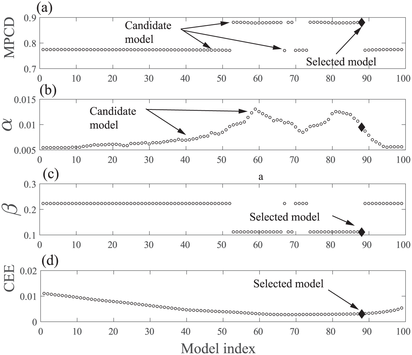
The goal is to select the candidate model with the highest MPCD. In the context of the problem that is being solved, the goal is to detect low-quality welds. Due to the relevance of failing to detect a potential defect, the type II error is the main concern of this analysis; for this reason, the MPCD is also used as a model selection criteria. The estimated MPCD, $α$ , $β$ , and validation error of each model are summarized in Figure 5.

Figure 5.

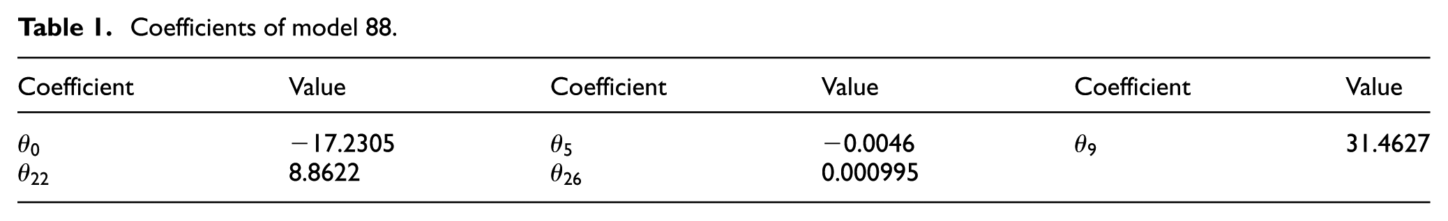
Generalization performance of candidate models: (a) validation MPCD, (b) validation $α$ , (c) validation $β$ , and (d) validation CEE.

According to the selection criteria, model 88 is the best candidate, with an estimated MPCD of 0.8805 ( $α = 0.0095$ , $β = 0.1111$ ) and four relevant features, and varying the values of $λ$ helped to identify the most relevant features. The coefficients are shown in Table 1. The value of $γ$ for this model is 0.0063, meaning that any value estimated by the logistic function below this threshold will be classified as 0 (i.e. good) or 1 (i.e. bad) otherwise.

Table 1.

Coefficients of model 88.

Coefficient	Value	Coefficient	Value	Coefficient	Value
$θ_{0}$	−17.2305	$θ_{5}$	−0.0046	$θ_{9}$	31.4627
$θ_{22}$	8.8622	$θ_{26}$	0.000995

According to the bias–variance analysis, Figures 3(d) and 5(d), the first candidate models (i.e. 1–60) exhibited over-fitting problems, while the last models (i.e. 91–99) exhibited under-fitting problems. Therefore, the bias–variance trade-off is efficiently overcome by this parsimonious candidate model.

A receiver operating characteristic (ROC) plot for model comparison efficiently depicts relative trade-offs between TP and FP. The best possible prediction method would be a point in the upper left corner, or coordinate 0, 1 of the ROC space; it would be a perfect classification. 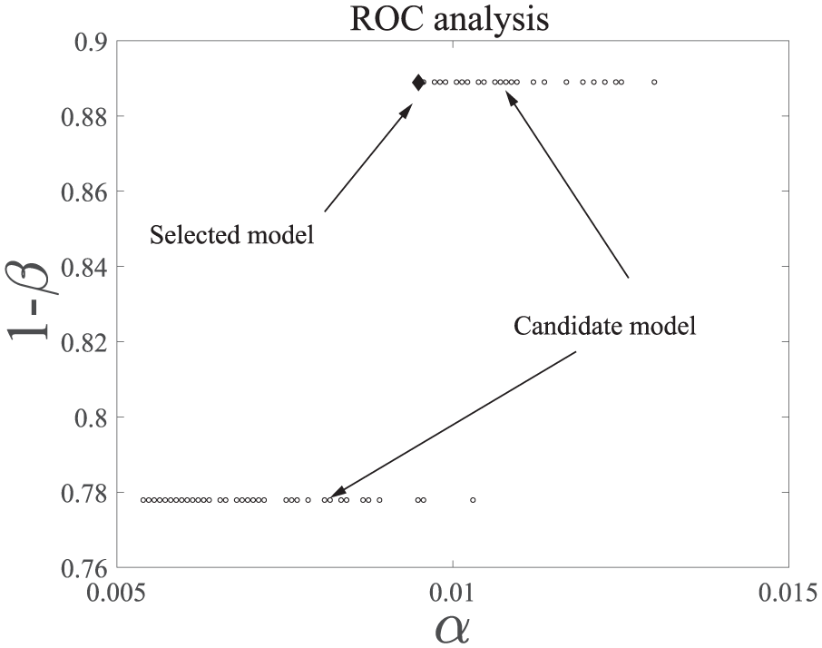The location of the chosen model in the ROC plot confirms that model 88 is the best candidate, and it has the smallest estimated $α$ from the set of candidate models with the same estimated $β$ . Figure 6 illustrates the relative location of the model 88 in the ROC curve.

Figure 6.

ROC curve of the candidate models.

Classifier assessment

The importance of this final step is to assess the classifier without the induced bias in the validation stage and to ensure the model satisfies the learning target. The estimated MPCD of the final model on the testing data is 0.9980 ( $β = 0$ , $α = 0.0020$ ). The testing set includes 10,000 records, with seven bad batteries. The classifier correctly classified the 7 bad units and only misclassified 20 good units. Recognition rates are summarized in Table 2.

Table 2.

Confusion matrix.

	Declare good	Declare bad
Good	9973	20
Bad	0	7

According to model assessment results, LR not only shows high prediction ability but also did not commit any type II error. The graphical representation of the classification using unseen data (i.e. testing set) is shown in Figure 7.

Figure 7.

LR-based classification.

LSW

To show the reproducibility and flexibility of the proposal, the same LP and PR strategy is applied to a balanced dataset, derived from an LSW process:

Laser welding is a welding technique used to join multiple pieces of metal through the use of a laser beam. The laser welding system provides a concentrated heat source, allowing for narrow, deep welds and high welding rates. This process is used frequently in high volume welding applications, such as in the automotive industry. Laser welding in the automotive industry has applications that enable manufacturers to weld component engine parts, transmission parts, alternators, solenoids, fuel injectors, fuel filters, air conditioning equipment, and air bags, as well as many other applications.⁴⁵

The LSW process is often completed in few milliseconds, it exhibits good repeatability and is easy to automate. It is an excellent option for high-productivity processes.

The dataset contains 2199 features and 317 examples (159 good, 158 bad), and it is partitioned following the hold-out validation scheme: training set (160), validation set (80), and test set (77). To maintain space efficiency, only the most relevant plots are included in this analysis.

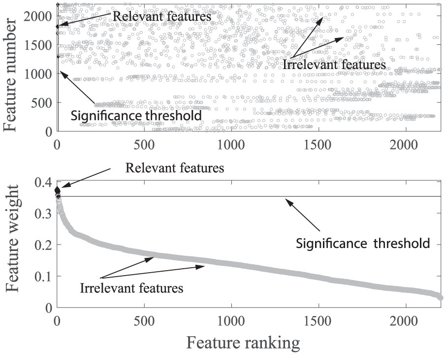
Since the included number of bad in this training set is significantly higher than the UMW dataset, the ReliefF algorithm is run with $k = 10$ , with a significance threshold of $τ = 0.3535$ . According to the ReliefF algorithm, feature 1812 is the most important feature, while feature 2190 is the feature with the least discriminative information. Figure 8 summarizes the feature ranking and which features are selected based on $τ$ . According to ReliefF, only 13 features—out of 2199—should be selected.

Figure 8.

Feature ranking and selection using Relief F.

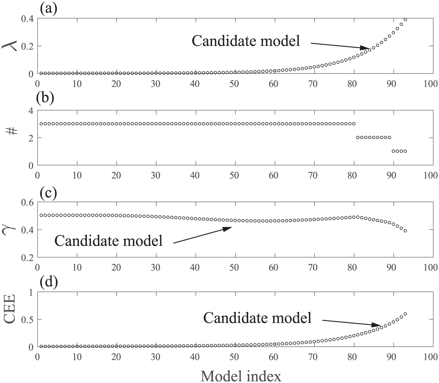
Redundant features from the subset obtained by ReliefF are eliminated by HCR algorithm using $δ = 0.90$ . The algorithm eliminated nine highly correlated features. Ultimately, the feature space was reduced to four relevant variables without high correlations. Then, the l₁-regularized LR algorithm was used to develop 93 candidate model. Figure 9(a)–(d) shows the most relevant information (e.g. $λ$ , number of features, $γ$ , training CEE, respectively) of each candidate model.

Figure 9.

Candidate model information: (a) values of λ, (b) number of features, (c) optical classification threshold, and (d) training CEE.

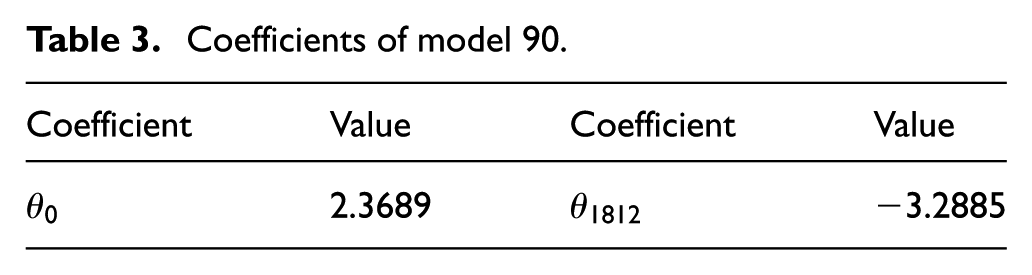
Since there are seven candidate models that perfectly separate the data 87–93, Figure 10(a), the number of features and the validation CEE are used as a secondary model selection criteria. Since models 90–93 contain only one feature, model 90 is chosen, since it is the candidate model with the smallest validation CEE, Figure 10(d). Coefficients are shown in Table 3, and its associated classification threshold is $γ = 0.4375$ , Figure 9(c).

Figure 10.

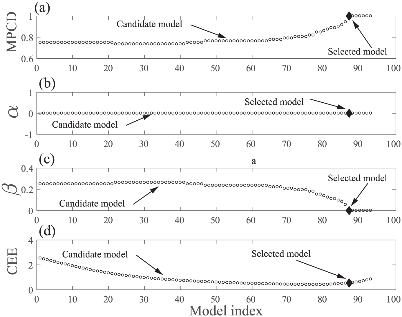
Generalization performance of candidate models: (a) validation MPCD, (b) validation α, (c) validation β, and (d) validation CEE.

Table 3.

Coefficients of model 90.

Coefficient	Value	Coefficient	Value
$θ_{0}$	2.3689	$θ_{1812}$	−3.2885

The selected model perfectly separated good from bad welds in the testing set. Recognition rates are summarized in Table 4 and graphically displayed in Figure 11.

Table 4.

Confusion matrix.

	Declare good	Declare bad
Good	50	0
Bad	0	27

Figure 11.

LR-based classification.

Comparative analysis

To evaluate the performance of the proposal, a comparative analysis is performed. The results of the two case studies were compared with a typical modeling analysis. The same learning algorithm was trained (with the same values of $λ$ ) without preprocessing the data and using widely known model selection approaches—CEE, AIC, and BIC.²⁴

Models were mainly compared based on their detection capacity with the smallest $α$ error possible; in addition, parsimony was also considered. Due to space constraints, only the most relevant graphs are presented.

UMW

Following the same data partition strategy, the training set is used to create the set of candidate models and to estimate the AIC and BIC scores. The associated number of features and the values of $γ$ (obtained using the OCTM algorithm) of each candidate model are displayed in Figure 12. While the validation set is used to estimate the MPCD and CEE of each model. Model selection results are summarized in Figure 13.

Figure 12.

Candidate model information: (a) number of features and (b) optimal classification threshold.

Figure 13.

Model selection approaches: (a) MPCD, (b) AIC model selection criterion, (c) BIC model selection criterion, and (d) CEE model selection criterion.

According to the AIC-BIC, candidate model 81 should be selected ( $AIC = 76.8137, BIC = 105.8712$ ), and this candidate model contains five features with an estimated MPCD of 0.8778. While the CEE criterion recommends model 69 ( $CEE = 0.0025$ ), and this model contains 16 features with an estimated MPCD of 0.7719. Table 5 summarizes the generalization performance in the testing set of the three selected models developed in this section and the final model from the UMW case study (e.g. final).

Table 5.

Generalization analysis of the selected models.

Model	Features	FP	TN	TP	MPCD
Final	4	20	9973	7	0.9980
Model 81	5	24	9969	7	0.9976
Model 69	16	14	9979	7	0.9986

FN: false negative; FP: false positive; TN: true negative; TP: true positive; MPCD: maximum probability of correct decision.

The three models correctly classified the seven bad units in the testing set with a very small $α$ . However, the final model contains only 4 features, while models 81 and 69 contain 5 and 16, respectively. From engineering perspective, it is significantly easier to interpret a model with 4 features than a model with 5 or 16.

LSW

Candidate model information is summarized in Figure 14, while the model selection criterion values are summarized in Figure 15.

Figure 14.

Candidate model information: (a) number of features and (b) optimal classification threshold.

Figure 15.

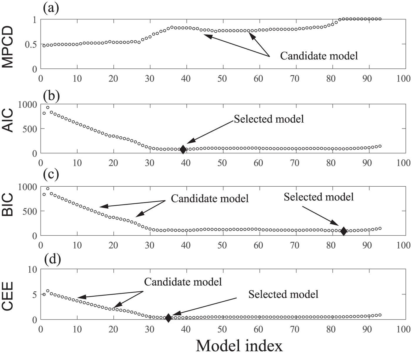
Model selection approaches: (a) MPCD, (b) AIC model selection criterion, (c) BIC model selection criterion, and (d) CEE model selection criterion.

According to the AIC, candidate model 39 should be selected ( $AIC = 72.2325$ ), and this candidate model contains 11 features with an estimated MPCD of 0.8194. While the BIC recommends candidate model 83 ( $BIC = 85.4445$ ) with only two features with an estimated MPCD of 1. Finally, the CEE criterion recommends model 35 ( $CEE = 0.2869$ ), and this model contains 14 features with an estimated MPCD of 0.8056. The generalization performance in the testing set is summarized in Table 6.

Table 6.

Generalization analysis of the selected models.

Model	Features	FN	TN	TP	MPCD
Final	1	0	50	27	1
Model 39	11	5	50	22	0.8148
Model 83	2	0	50	27	1
Model 35	14	6	50	21	0.7778

FN: false negative; FP: false positive; TN: true negative; TP: true positive; MPCD: maximum probability of correct decision.

In this case study, the final model outperforms the three models, although model 83 perfectly separates the classes, and this model contains two features. However, models 39 and 35 have many features and also failed to detect all the bad units; therefore, the MPCD is significantly lower.

Discussion

Based on the comparative analysis, the models developed following the proposed LP and PR strategy exhibited better parsimony properties and good (or even better) detection capacity when compared with a typical l₁-regularized LR analysis with three popular model selection criterion (e.g. AIC, BIC, and CEE).

Although l₁-regularized LR learning algorithm induces sparsity, the proposed strategy can boost the learning algorithm by eliminating irrelevant and redundant features.

The same approach is also being applied to different automotive manufacturing systems with promising results; however due to space constraints, they are not discussed in this article.

Conclusion

Today’s business environment sustains mainly those companies committed to a zero-defect policy. This quality challenge was the main driver of this research, where an LP and PR strategy was developed for a KB ISCS. The proposed approach was aimed at detecting rare quality events in manufacturing systems and to identify the most relevant features to the quality of the product. The defect detection was formulated as a binary classification problem and validated in two experimental datasets derived from automotive manufacturing systems: (1) UMW of battery tabs from a battery assembly process and (2) LSW sub-assembly components from an assembly process. In both cases, the main objective was to detect low-quality welds (bad) from the process.

To increase the classifier prediction ability and reduce training times, the dataset was preprocessed in a two-step approach: (1) the ReliefF algorithm was used to eliminate irrelevant features, and (2) the HCR algorithm was applied to eliminate redundant features that most filter methods cannot eliminate.

The l₁-regularized LR was used as the learning algorithm for the classification task and to identify the most important features. Since the form of the model was not known in advance, a set of candidate models was developed—by varying the value of $λ$ —as an effort to approximate the true model. Chosen model exhibited high capacity to detect rare quality events, since 100% of the defective units on the testing set were detected.

The proposed strategy used the MPCD as a model selection criterion. Therefore, the OCTM algorithm was developed to find $γ$ , the optimal classification threshold with respect to MPCD.

The proposed approach can be adapted and widely applied to manufacturing processes to boost the performance of traditional quality methods and potentially move quality standards forward, where soon virtually no defective product will reach the market.

Future work

Since MPCD is founded exclusively on recognition rates, future research along this path could focus on adding a penalty term for model complexity. Although information-theoretic approaches such as AIC and BIC penalize for model complexity, they are not mainly founded on recognition rates.

Footnotes

Appendix 1

The HCR algorithm has three components, Figure 16:

The algorithm performs $n$ iterations (lines 1, 2, 12, and 13) to find which features are highly correlated to feature $i$ , and the $CorrFeat$ variable is updated and evaluated at each iteration, with three possible scenarios: (1) when feature $i$ does not have any correlated features and has not been previously evaluated, that feature is added to the $SUFL$ and $TabuList$ (lines 3 and 4); (2) when feature $i$ has one or more highly correlated feature(s) and is not in the $TabuList$ , that feature is added to the $SUFL$ , while the highly correlated features larger than $i$ are added to the $EliminatedList$ , maintaining the uniqueness of the elements in the $EliminatedList$ while updating the $TabuList$ (lines 5–9); and (3) otherwise, the three sets are unchanged (lines 10 and 11).

Since the best values of $k$ —for ReliefF—and $δ$ —for HCR—are not known in advance, they can be tuned with respect to prediction. The value of $k$ can be set based on the number of bad units in the training, and $δ$ can be heuristically set and evaluated between 0.50 and 0.95.

Appendix 2

The OCTM algorithm has three components, Figure 17:

The algorithm performs $m - 1$ iterations (lines 1 and 5) to find the candidate classification thresholds (line 2), $CC T_{i}$ , $i = 1, . . ., m - 1$ . The $MPC D_{i}$ is estimated at each $CC T_{i}$ (line 3). The candidate classification threshold list is $CCTL = {MPC D_{i}}_{i = 1}^{m - 1}$ (line 4). Find the position $p$ of the maximum value of $CCTL$ . Finally, $γ$ is the value of $CC T_{p}$ (lines 6 and 7).

Acknowledgements

We would like to express our deepest appreciation to Dr Debejyo Chakraborty, Diana Wegner, and Dr Xianfeng Hu, who helped us to complete this report. A special gratitude is given to Dr Jeffrey Abell, whose ideas and contributions illuminated this research.

Handling Editor: Baozhen Yao

Declaration of conflicting interests

The author(s) declared no potential conflicts of interest with respect to the research, authorship, and/or publication of this article.

Funding

The author(s) disclosed receipt of the following financial support for the research, authorship, and/or publication of this article: This work was partially supported by the Consejo Nacional de Ciencia y Tecnologia (CONACYT; under grant 404325/215143).

References

AS of Quality. Emergence—2011 future of quality study. Milwaukee, WI: ASQ: The Global Voice of Quality, 2011.

Schwab

. The fourth industrial revolution: what it means, how to respond. World Economic Forum, 2016, https://www.weforum.org/agenda/2016/01/the-fourth-industrial-revolution-what-it-means-and-how-to-respond/

Yin

Kaynak

. Big data for modern industry: challenges and trends. Proc IEEE 2015; 103: 143–146.

Yin

Gao

et al . Data-based techniques focused on modern industry: an overview. IEEE T Ind Electron 2015; 62: 657–667.

Venkatasubramanian

Rengaswamy

Kavuri

et al . A review of process fault detection and diagnosis: part III: process history based methods. Comput Chem Eng 2003; 27: 327–346.

Escobar

Morales-Menendez

. Machine learning and pattern recognition techniques for information extraction to improve production control and design decisions. In: Proceedings of the advances in data mining, ICDM 2017 (ed P

Perner

), New York, 12–13 July 2017, pp.285–295, Berlin: Springer.

Ghosh

. A comparative roundup: artificial intelligence vs. machine learning vs. deep learning, June 2016, www.dataversity.net/ai-vs-machine-learning-vs-deep-learning

Theodoridis

Koutroumbas

. Pattern recognition and neural networks. In: Paliouras

Karkaletsis

Spyropoulos

(eds) Machine learning and its applications. Berlin: Springer, 2001, pp.169–195.

Zhou

. Ensemble learning. In: Li

Jain

(eds) Encyclopedia of biometrics. Berlin: Springer, 2009, pp.270–273.

10.

Bishop

. Pattern recognition and machine learning. Berlin: Springer, 2006.

11.

Bradley

Mangasarian

. Feature selection via concave minimization and support vector machines. In: Proceedings of the machine learning 15th international conference, 24–27 July, 1998, pp.82–90. San Francisco, CA: Morgan Kaufmann.

12.

Liu

. Feature selection for high-dimensional data: a fast correlation-based filter solution. In: Fawcett

Mishra

(eds) Proceedings of the 20th international conference on machine learning, Washington, DC, 21–24 August 2003, pp.856–863.

13.

Hall

. Correlation-based feature selection of discrete and numeric class machine learning. In: Proceedings of the 17th international conference on machine learning, 29 June–2 July 2000, pp.359–366. Hamilton, New Zealand: University of Waikato.

14.

Nicodemus

Malley

. Predictor correlation impacts machine learning algorithms: implications for genomic studies. Bioinformatics 2009; 25: 1884–1890.

15.

Wang

Yang

et al . Feature selection using feature ranking, correlation analysis and chaotic binary particle swarm optimization. In: Proceedings 5th IEEE international conference on software engineering and service science, Beijing, China, 23 October 2014, pp.305–309. New York: IEEE.

16.

Shao

Paynabar

Kim

et al . Feature selection for manufacturing process monitoring using cross-validation. J Manuf Syst 2013; 32: 550–555.

17.

Wang

et al . Application of global optimization methods for feature selection and machine learning. Math Probl Eng. Epub ahead of print 2 September 2013. DOI: 10.1155/2013/241517.

18.

Kira

Rendell

. The feature selection problem: traditional methods and a new algorithm. In: Proceedings of the 10th national conference on artificial intelligence, San Jose, CA, 12–16 July 1992, vol. 2, pp.129–134. New York: ACM.

19.

Chandrashekar

Sahin

. A survey on feature selection methods. Comput Electr Eng 2014; 40: 16–28.

20.

Robnik-Šikonja

Kononenko

. Theoretical and empirical analysis of ReliefF and RReliefF. Mach Learn 2003; 53: 23–69.

21.

Bishop

. Neural networks for pattern recognition. Oxford: Oxford University Press, 1995.

22.

. Feature selection L1 vs L2 regularization and rotational invariance. In: Proceedings of the 21st international conference on Machine learning, Banff, AB, Canada, 4–8 July 2004, p. 78. New York: ACM.

23.

Xing

Jordan

Karp

. Feature selection for high-dimensional genomic microarray data. In: Proceedings of the 18th international conference on machine learning ICML, Williamstown, MA, 28 June–01 July 2001, vol. 1, pp.601–608. San Francisco, CA: Morgan Kaufmann.

24.

Peruggia

. Model selection and multimodel inference: a practical information-theoretic approach. J Am Stat Assoc 2003; 98: 778–779.

25.

Fawcett

. An introduction to ROC analysis. Pattern Recog Lett 2006; 27: 861–874.

26.

Friedman

Hastie

Tibshirani

. The elements of statistical learning, vol. 1: Berlin: Springer, 2001.

27.

Devore

. Probability and statistics for engineering and the sciences. Boston, MA: Cengage Learning, 2015.

28.

Lee

Abbeel

et al . Efficient L1 regularized logistic regression. In: Proceedings of the national conference on artificial intelligence, Cambridge, MA, 16–20 July 2006, p. 401. Reston, VA: AIAA.

29.

Murphy

. Machine learning: a probabilistic perspective. Cambridge, MA: The MIT Press, 2012.

30.

Tibshirani

. Regression shrinkage and selection via the Lasso. J Roy Stat Soc Ser B Met 1996; 58: 267–288.

31.

Zhao

. On model selection consistency of Lasso. J Mach Learn Res 2006; 7: 2541–2563.

32.

Uraikul

Chan

Tontiwachwuthikul

. Artificial intelligence for monitoring and supervisory control of process systems. Eng Appl Artif Intel 2007; 20: 115–131.

33.

Chiang

Braatz

Russell

. Fault detection and diagnosis in industrial systems. Berlin: Springer Science+Business Media, 2001.

34.

Huan

Motoda

. Feature extraction, construction and selection: a data mining perspective. Berlin: Springer Science+Business Media, 1998.

35.

Luiz

Lorena

André

et al . Filter feature selection for one-class classification. J Intell Robot Syst 2015; 80: 227–243.

36.

Khan

Madden

. A survey of recent trends in one class classification. In: Proceedings of the Irish conference on artificial intelligence and cognitive science, Dublin, Ireland, August 2009, pp.188–197. Berlin: Springer.

37.

Manevitz

Yousef

. One-class SVMs for document classification. J Mach Learn Res 2001; 2: 139–154.

38.

Abell

Chakraborty

Escobar

et al . Big data driven manufacturing—process-monitoring-for-quality philosophy. J Manuf Sci Eng. Epub ahead of print 31 January 2017. DOI: 10.1115/1.4036833.

39.

Abell

Spicer

Wincek

et al . Binary classification of items of interest in a repeatable process. Patent US8757469B2, June 2014, www.google.com/patents/US20130105556

40.

Wolpert

. The lack of a priori distinctions between learning algorithms. Neural Comput 1996; 8: 1341–1390.

41.

Tibshirani

. Statistical learning with sparsity: the lasso and generalizations, vol. 79. Boca Raton, FL: CRC Press, 2014.

42.

Natrella

. NIST/SEMATECH e-handbook of statistical methods, 2010, http://www.itl.nist.gov/div898/handbook/

43.

Zhu

Rosset

Hastie

et al . 1-norm support vector machines. Adv Neur In 2004; 16: 49–56.

44.

Fung

Mangasarian

. A feature selection Newton method for support vector machine classification. Comput Optim Appl 2004; 28: 185–202.

45.

Subhajit

. Laser welding: a new dimension in auto-motive industry. OEM Update, December 2016, www.oemupdate.com/industry-update/*-industry

Machine learning techniques for quality control in high conformance manufacturing environment

Abstract

Keywords

Introduction

Theoretical background

ML and PR

Feature space reduction

FS

Regularization

Classifier design, selection, and assessment

CM

LR

ISCS

LP and PR strategy

LP

Discussion

Case studies

UMW

Feature space reduction

Classifier design

OCTM

Classifier selection

Classifier assessment

LSW

Comparative analysis

UMW

LSW

Discussion

Conclusion

Future work

Footnotes

Appendix 1

Appendix 2

Acknowledgements

Declaration of conflicting interests

Funding

References