Recognition of partial scanning low-level wind shear based on support vector machine

Abstract

A majority of air crash is caused by low-level wind shear. That can affect the direction and velocity of the aircrafts. So, it is very necessary to recognize the low-level wind shear in a short time to make the early warning. In this article, we propose a recognition method which uses support vector machine to make the classification of the low-level wind shear images measured by laser detection and ranging. We use the partial scanning images instead the traditional whole scanning ones, so that it can decrease the calculation time and avoid the wind field inversion. The feature exacting methods we use are invariant moments and gray-gradient co-occurrence matrix. They can, respectively, catch 7 features and 15 features of the wind velocity distribution images. At the same time, we use support vector machine that the parameters are optimized by K-fold cross-validation to do the pattern recognition. Moreover, the simulation results of recognition are given.

Introduction

In atmospheric wind field data, low-level wind shear is one of the meteorological phenomena and has great harm. It greatly affects the takeoff and landing safety of aircrafts and is one of the main causes of aviation disaster. In general, low-level wind shear refers to the sudden change in wind velocity below 600 m in the air. If the aircraft cannot resist wind shear, it will lead to stall or even crash. Therefore, the early warning of the low-level wind shear is very necessary. In 1982, the joint airport weather study confirmed the possibility of detection the microburst by Doppler radar. ¹ In 1987, SD Campbell and S Olson ² proposed for the first time to use the artificial intelligence method to recognize the wind shear. After 1993, Delanoy and his group began to use a machine learning method to recognize the low-level wind shear. This method was used in the airport surveillance radar system and next-generation weather radar system. ³ Those methods used the traditional radar data and needed to do the wind field inversion. They needed a huge computation and calculated slowly. In recent years, laser detection and ranging (lidar) has been used to detect the low-level wind shear. It has high resolution, better performance and capability of anti-jamming. A lot of methods have been used to detect the wind field. Wind field inversion is the most common method that uses the mathematical principle to calculate three-dimensional (3D) wind field by the radial wind velocity measured by lidar. However, this method needs a plenty of scanning data and has low calculation speed. It is not convenient for early warning. Lihui Jiang and his group used image recognition methods to identify the class of the low-level wind shear. The images they used were the wind velocity distribution measured by the lidar. The idea they proposed can reduce the recognition time greatly.^4–7

However, in order to get the real-time detection, we need to reduce the scanning time of the lidar. In this article, we propose a new recognition system that uses partial scanning image to compose the image samples. Different kinds of methods have been used to do the pattern recognition. Such as neural networks, genetic algorithm, and support vector machine (SVM). Neural network is a mathematical model that imitates the behavioral characteristics of animals and can process the distributed parallel information. It has strong ability of nonlinear filtering, strong robustness, and can map any complex nonlinear relationship.^8,9 A few of nonlinear filtering methods are proposed to solve the related problems, such as distributed moving horizon state estimation and switching communication channels.^10–13 Genetic algorithm is a computational model for simulating the Darwin’s natural selection and genetic mechanism. It is a method to search the optimal solution by simulating the natural evolutionary process. This algorithm has a powerful ability of fault tolerance and is fit for any search spaces. But, neural networks and genetic algorithm are not very suitable for the recognition of less samples. Therefore, in this article, we choose the SVM method to recognize the wind shear classes, because it has better adaptability of less partial samples.

Basic theory of low-level wind shear

Low-level wind shear mainly includes microburst, side wind shear, tailwind-or-headwind wind shear, and low-level jet stream. The microburst refers to a situation in which the aircraft enters a strong descending airflow area from a no obvious descending airflow area, which has more intense impacts and can cause a sudden sinking of the airplane. Side wind shear refers to the wind-level mutation on the side of the aircraft. It will cause yaw, side slip, and roll of the aircraft. Low-level jet stream refers to the airflow mutation of low-level atmosphere. It is a narrow strong wind zone in a short period of time. The regional wind field will suddenly change when the low-level stream is coming. Tailwind-or-headwind wind shear refers to the situation of tailwind suddenly increasing or headwind decreasing. It will change the lift force of the aircrafts. In this article, we use software named Fluent, which is a famous fluid mechanics simulation tool, to simulate the low-level wind shear over the ocean. The position of lidar is shown in Figure 1.

Figure 1.

The position of lidar on the ship.

We will get two kinds of scanning data. One is called plane position illustrate (PPI), and the other one is called ranging height illustrate (RHI). The decision of the parameters is shown in Table 1. In Table 1, α means the pitch angle, β is the angle between the PPI image, and x-axis. γ means the angle between the RHI image and x-axis, δ is the angle between the RHI image and z-direction. A part of the simulation results is shown in Figures 2 and 3. They show the whole scanning of the PPI and RHI.

Table 1.

The parameters of scanning data.

Distance	α	β	γ	Δ
120 (m)	0°, 3°, 5°	[180°, 360°]	180°, 225°,315°, 360°	[30°, 90°]

Figure 2.

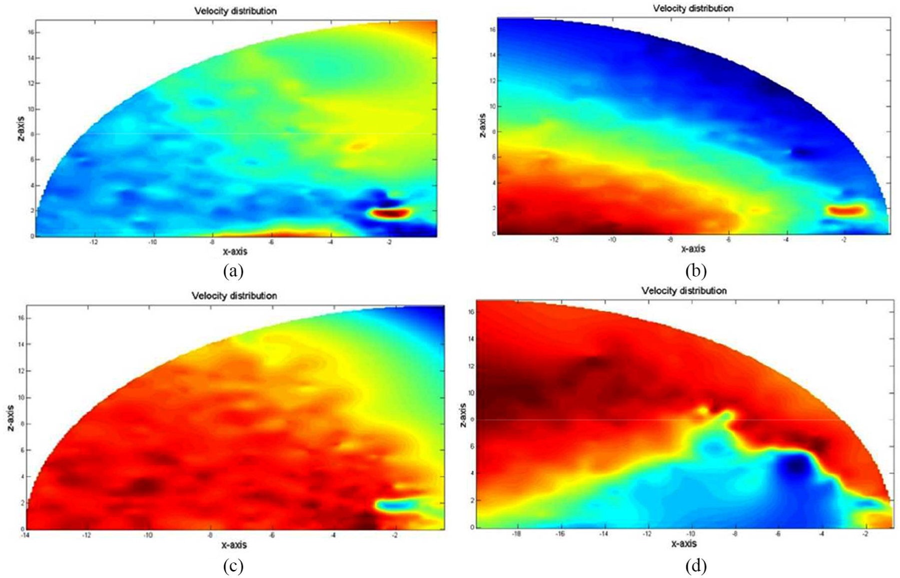
The whole scanning PPI velocity distribution of low-level wind shear: (a) side wind shear, (b) microburst, (c) low-level jet stream, and (d) tailwind-or-headwind wind shear.

Figure 3.

The whole scanning RHI velocity distribution of low-level wind shear: (a) side wind shear, (b) microburst, (c) low-level jet stream, and (d) tailwind-or-headwind wind shear.

Even though the whole scanning images can reveal more features, it needs more time to calculate. So, in this article, we aim to recognize the low-level wind shear by partial scanning images. That can decrease the processing time and will be closer to the real-time detection. Figures 4 and 5 show some of the partial scanning images.

Figure 4.

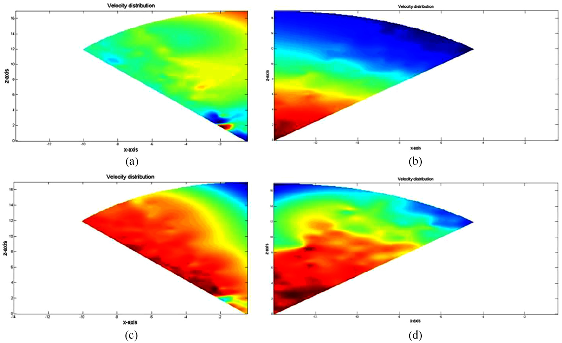
The partial scanning PPI velocity distribution of low-level wind shear: (a) side wind shear, (b) microburst, (c) low-level jet stream, and (d) tailwind-or-headwind wind shear.

Figure 5.

The partial scanning RHI velocity distribution of low-level wind shear: (a) side wind shear, (b) microburst, (c) low-level jet stream, and (d) tailwind-or-headwind wind shear.

The feature exacting

Before presenting the pattern recognition of the wind shear images, we need to exact the features. In this article, we use the invariant moment method and gray-gradient co-occurrence matrix to get the edge features and texture features of the images.

Invariant moment

We use a theory of two-dimensional (2D) invariant moment to exact the features of the images. In the methods of feature exacting, the invariant moment is widely used because it has nature of rotation, proportion, and translation. For an M × N pixels image f(i, j), the decision for the (p+q) order moment of inertia is

$$m_{\mathrm{pq}}=\sum _{i=1}^M\sum _{j=1}^N{i}^p{j}^{q}f(i,j)$$

(1)

The center of gravity is decided by

$$\overline{i}=m_{10}\sum _{i=1}^M\sum _{j=1}^{N}if(i,j),\overline{j}=m_{01}\sum _{i=1}^M\sum _{j=1}^{N}jf(i,j)$$

(2)

The (p + q) order moment of center is decided by

$${\mu }_{\mathrm{pq}}=\sum _{i=1}^M{\sum _{j=1}^N(i-\overline{i})}^p{(j-\overline{j})}^{q}f(i,j)$$

(3)

The seven invariant moments are deduced by the normalized center moment. The following six are absolute orthogonal invariants

$${\varphi }_1={\eta }_{20}+{\eta }_{02}$$

(4)

$${\varphi }_2={({\eta }_{20}+{\eta }_{02})}^2+4{\eta }_{11}^2$$

(5)

$${\varphi }_3={({\eta }_{30}-3{\eta }_{12})}^2+{(3{\eta }_{21}-{\eta }_{03})}^2$$

(6)

$${\varphi }_4={({\eta }_{30}+{\eta }_{12})}^2+{({\eta }_{21}+{\eta }_{03})}^2$$

(7)

$$\begin{array}{c}\multicolumn{1}{c}{{\varphi }_5=(3{\eta }_{21}-{\eta }_{03})({\eta }_{21}+{\eta }_{03})[{({\eta }_{30}+{\eta }_{12})}^2-{({\eta }_{21}+{\eta }_{03})}^2]}\\ \multicolumn{1}{c}{+({\eta }_{30}-3{\eta }_{12})({\eta }_{30}+{\eta }_{12})[{({\eta }_{30}+{\eta }_{12})}^2-3{({\eta }_{21}+{\eta }_{03})}^2]}\end{array}$$

(8)

$$\begin{array}{cc}\multicolumn{1}{c}{{\varphi }_6=}& (3{\eta }_{21}-{\eta }_{03})[{({\eta }_{30}+{\eta }_{12})}^2-{({\eta }_{21}+{\eta }_{03})}^2]\hfill \\ \multicolumn{1}{c}{}& +4{\eta }_{11}({\eta }_{30}+{\eta }_{12})({\eta }_{21}+{\eta }_{03})\hfill \end{array}$$

(9)

and one skew orthogonal invariants

$$\begin{array}{c}\multicolumn{1}{c}{{\varphi }_7=(3{\eta }_{21}-{\eta }_{03})({\eta }_{30}+{\eta }_{12})[{({\eta }_{30}+{\eta }_{12})}^2-3{({\eta }_{21}+{\eta }_{03})}^2]}\\ \multicolumn{1}{c}{-({\eta }_{30}-3{\eta }_{12})({\eta }_{21}+{\eta }_{03})[3{({\eta }_{30}+{\eta }_{12})}^2-{({\eta }_{21}+{\eta }_{03})}^2]}\end{array}$$

(10)

Using equations (4)–(10), we can calculate the features of the wind velocity images. ¹⁴

Gray-gradient co-occurrence matrix

Gray-gradient co-occurrence matrix is a kind of feature exacting method that uses the gray scale and gradient to catch the texture characteristics of the image. The element of the matrix H(i, j) is decided by the pixel points number of the normalized gray image F(m, n) and gradient image G(m, n) that gray scale is i and gradient is j. In total, 15 features can be obtained from this matrix. We assume the Gray-gradient co-occurrence matrix is C, and its element is c_ij. Then, the probability when the gray scale equals to i and gradient equals to j of the matrix C is shown

$$p_{\mathrm{ij}}=\frac{c_{\mathrm{ij}}}{\sum _i\sum _j{c}_{\mathrm{ij}}}$$

(11)

To calculate the digital features of the matrix C, we can get the texture features of the image. Common digital features of gray-gradient co-occurrence matrix are the energy, the average of gray scale, the average of gradient, the mixed entropy, and the deficit moment. We can get 15 features of the image using the gray-gradient co-occurrence matrix method. ¹⁵

Image recognition based on SVM

SVM is a well-known classifier because it has excellent accuracy. It is proposed to solve the classification between two classes. Its basic idea is to search a best hyper plane to identify the different classes with better classification accuracy. A kernel function is used to do the nonlinear transformation to change the input space to a high-dimensional space. Then, we search the best classification plane in this space, so that it is not easy to fall into the local optimal value.^16–18 In this article, we choose a K-fold cross-validation (K-CV) method to optimize the parameters of SVM, so that the accuracy can be improved. Its main idea is to divide the data into K groups. Each group composes the test data respectively, and the other K – 1 groups compose the training data. Then, we use the K results to be the performance to optimize the classifier parameter. ¹⁹ The simulation result without optimization is shown in Figures 6 and 7.

Figure 6.

The labels and feature distribution: (a) invariant moments, (b) gray-gradient co-occurrence matrix, and (c) mixing features.

Figure 7.

The recognition result: (a) invariant moments, (b) gray-gradient co-occurrence matrix, and (c) mixing features.

Figure 6 shows the labels distribution and feature distribution of the training samples. There are 200 images, and each class get 50 ones. The feature distribution includes three kinds of result, the first is from invariant moments, the second one is from gray-gradient co-occurrence matrix, and the last is from the mixing of the first two methods. We only show seven features of each kind. Figure 7 shows the recognition results that computed by SVM with three different kinds of features. The red star means the classification result by SVM, and the blue circle means the real class of the testing samples. Table 2 shows the classification accuracy.

Table 2.

Classification accuracy of three methods by SVM.

Featureexacting	Invariant moments	Gray-gradientco-occurrencematrix	Mixing
Accuracy (%)	25.6579	26.3158	28.9474

Because our purpose is to reduce the recognition time, we use partial scanning images instead of the whole scanning ones, the accuracy of classification is a little low. As we all know, the designing focus of SVM is the choosing of kernel function. Kernel function changes the input data to a high-dimensional space, so that the hyper plane can be searched. So, we use the K-CV method to optimize parameters c and g. That c refers to the penalty factor, and g refers to the kernel parameter. The K-CV method can help to choose the best c and g, so that we can get best recognition accuracy. Table 3 reveals the optimized result by K-CV method.

Table 3.

Optimized result by K-CV method.

Feature exacting	Invariantmoments	Gray-gradientco-occurrencematrix	Mixing
Accuracy (%)	45.5	40.5	50
Best c	32	32	32
Best g	8	32	16

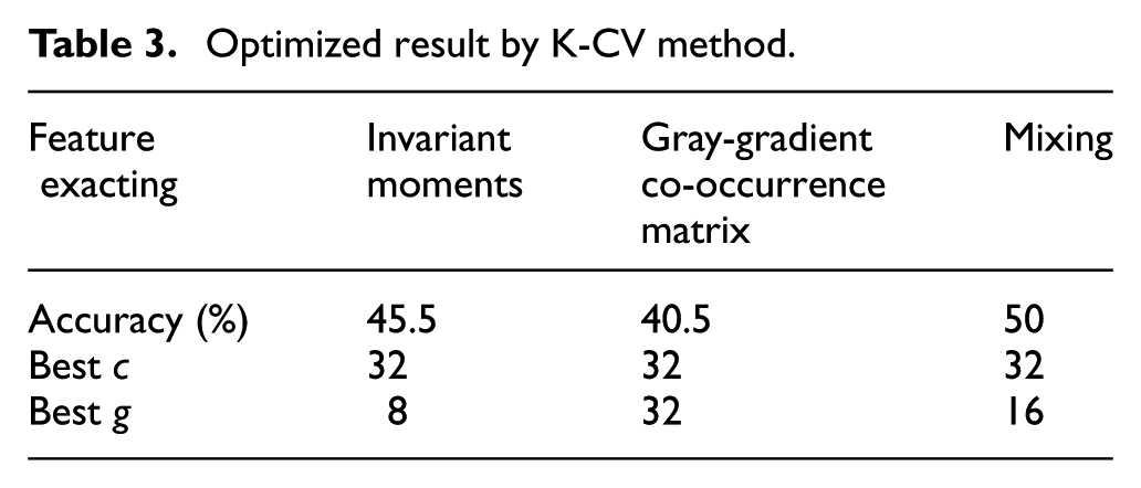
From Table 3, we can find the recognition accuracy has an obvious improvement after using the K-CV method to decide the parameters of SVM. But the accuracy is still lower than 50%, because the images we have used are from partial scanning. It is more different from other research and will save much time. In the future, we can use some filter to remove the noise and make the clutter suppression of the images. Such as the finite impulse response (FIR) filter which can guarantee the arbitrary amplitude–frequency characteristics and have strict linear phase–frequency characteristics. While this filter is a stable system and its unit sampling response is limited long.^20–22 So the recognition accuracy can be improved.

Conclusion

In this article, a partial scanning low-level wind shear recognition mode is proposed to recognize the class of wind shear to realize the real-time early warning. The images are simulated by the software Fluent. Two scanning modes named PPI and RHI are given to get the wind shear images. The invariant moments, gray-gradient co-occurrence matrix, and the mixing of those two are used to exact the features of the image samples. A machine learning method named SVM optimized by K-CV method is used to do the classification. The accuracy rate of the partial scanning mode is given by simulation. It is not perfect compared with whole scanning mode. However, the partial scanning time is just about 1/3 of the whole scanning time. And, this can save much more time and computation than the method by wind field inversion. It is very significant for the early warning of the low-level wind shear during the takeoff and landing of aircrafts.

In the future, more details and new methods should be added to improve the recognition accuracy rate to realize the real-time early warning of low-level wind shear.