
Abstract
Accurate sales forecasting plays an increasingly important role in automobile companies due to fierce market competition. In this article, an econometric model is proposed to analyze the dynamic connections among Chinese automobile sales, typical domestic brand automobile (Chery) sales, and economic variables. Four tests are required before modeling, which include unit root, weak exogeneity, cointegration, and Granger-causality test. The selected economic variables consist of consumer confidence index, steel production, consumer price index, and gasoline price. Monthly is used to empirical analysis and the result shows that there is long-term cointegration relationship between Chinese automobile sales and the endogenous variables. A vector error correction model in econometric based on cointegration is applied to quantify long-term impact of endogenous variables on Chinese automobile sales. Compared with other classical time-series methods, root mean square error (0.1243) and mean absolute percentage error (10.2015) by vector error correction model for 12-period forecasting are minimal. And the forecasting result is better when the impact of Chery sales is considered. That means that the fluctuation trends of Chinese automobile sales and typical domestic brand automobile sales are closely linked.
Keywords
Introduction
Accurate sales forecasting plays a crucial role in the competition of automobile market, and the automobile manufacturers need to forecast sales to achieve desired objectives. The prediction accuracy directly affects firms on judging the pattern of market demand, identifying the competitive strengths and determining product developmental strategies.1–5 There are many factors that affect automobile sales, and there is an inherent correlation among them. The time-series model can deeply analyze the internal relation between two parameters. Vector auto-regression (VAR) model can reflect the interrelationships among variables, embodying the effects of late lag and perturbation in any period on individual variables. The vector error correction model (VECM) also can reflect the dynamic process of adjusting from short-term departure to the long-term equilibrium among the variables. In addition, VECM can determine the theoretical relationship among variables in the model. Compared with traditional mathematical statistics and econometric methods, the VECM has the unique advantages in analyzing the time sequence data generated by non-stationary processes.6–9
Currently, the auto-regressive moving average (ARMA) model in the time-series model is commonly used to forecast future demand. Chen et al. 10 proposed a method based on ARMA model to forecast the demand for automobile spare parts, in which the case study used the sales data of a 4s shop in Shanghai. Hong and Bo 11 considered the short of circle and irregular factor in multiplication model and used the ARMA (1,1) model to forecast the circle and irregular factor separated from multiplication model. However, the model is explained by its own past information or lag values and random perturbations, taking no account of the impacts of economic variables on automobile sales. It is necessary to add the economic variables into the automobile sales forecasting, and the effectiveness of influence factors has been verified. Kitapcı et al. 12 analyzed the effect of economic policies applied to automobile sales using multiple regression and neural network methods, in which considered GDP, the rate of inflation, new car price index, and the euro exchange rate. Brühl et al. 13 proposed a forecasting model based on time-series analysis and data mining methods, which selected GDP, the gasoline prices, unemployment rate, interest rate, and consumer price index (CPI). In recent years, the domestic brand automobiles have developed rapidly and automobile manufacturers have accumulated a lot of experience. Their manufacturing and research capabilities continue to improve. Gradually, more and more consumers accept domestic brand automobiles. During the past few years, Chery has been China’s own brand sales champion and has become a representative of China’s own brands. In other words, the sales of Chery are very representative. Therefore, we can suppose boldly that the fluctuation trends of Chinese automobile sales and domestic brand automobile sales may be closely linked. However, considering the brand automobile sales, especially domestic brand automobile sales into the automobile sales forecasting at present, is indeed rare. Therefore, some economic variables are employed in this article, and then, the influence of the domestic typical brand automobile sales (Chery) on sales is taken into consideration to forecast Chinese automobile sales. Finally, the two forecasting performances of considering the influence of Chery sales and ignoring it are considered. Dekimpe et al. 6 and Sa-ngasoongsong et al. 14 thought that VAR and VECM are powerful, which are theory-driven models that can be used to describe the long-run dynamic behavior of multivariate time series. In addition, VAR and VECM in the time-series model are introduced in this article, and then, their forecasting performances are compared.
In the following section, the selection of economic variables is briefly described. The basic VAR and VECM algorithms are given in section “The theory of VAR and VECM.” In section “Model and implementation details,” proposed four tests are explained. In section “The evaluation of forecasting performance,” the establishment of the forecasting model, the stability of the models test and the results obtained by automobile sales forecasting model, and comparisons with VAR and ARMA are presented. Finally, the conclusion of this study is given in section “Conclusion.”
Data
In this article, the data are divided into three parts, which includes Chinese automobile sales, Chery sales, and the selected economic variables. Chery sales which contribute to Chinese automobile sales have a larger share in automobile market of China. The data that used the monthly data from 2007 to 2016 are used, which are collected from the National Bureau of Statistics and SOHU Automobiles in China. The trends of Chinese automobile sales and Chery sales in China are shown in Figures 1 and 2, respectively. Next, the selection of economic indicators is the remaining task. The purpose of adding economic variables is to improve the efficiency of automobile sales forecasting and the convenience of structural relationship analysis among variables. The characteristics of economic variables considered in this article are as follows:
Variables that describe the changes in the price paid by automobile consumers.
Variables that affect the automobile sales demand.
Variables that reflect the changes in national economy and the economic cycle.

The trend of Chinese automobile sales.

The trend of Chery sales in China.
Beyond that, when choosing the economic variables, some issues including multicollinearity, over-parameterization, and model specification and so on should be considered. Based on the literature reference and some experiments, four economic variables are selected in this article: consumer confidence index (CCI), steel production, CPI, and 95# unleaded gasoline price (hereafter referred to as gasoline price).14–16 The data are collected from the National Bureau of Statistics and CNII with a time horizon of months to forecast. The econometric model is presented to identify the structural relationship among automobile sales, Chery sales, and these economic variables.
Table 1 summarizes the data of Chinese automobile sales, Chery sales, and the selected economic variables. In order to improve the efficiency of modeling and validation, a partial sample from January 2007 to December 2015 is used to develop the model, and the remaining data are used to validate.
Summary of variables.

CCI: consumer confidence index; CPI: consumer price index.
The theory of VAR and VECM
VAR is a natural extension of the univariate auto-regression (AR) model, which is based on the statistical properties of the data. The univariate auto-regression model is exploited to VAR with multivariate time series since each endogenous variable is known as the function of the lag value of the endogenous variable in the model. VAR can also receive feedback from each endogenous variable, and the feedback can reflect the structural relationships among variables in the model. VAR is one of the models that are easy to operate in the analysis and prediction among multiple related economic indicators. A pth-order VAR, denoted as VAR(p), can be represented as 14

where yt = (y1t·… yNt) denotes a N − 1 dimensional time-series vector;
When there are unit roots in VAR for the exogenous variables, the VAR in difference form is stationary and may be more reasonable. But it is not the best choice since the VAR in difference form will lose some disequilibrium information that is important. The cointegration relationship among variables reflects the long-term relationship among variables. Furthermore, unbalanced error and the variables in difference form are also used to establish a stationary VAR model, thus an important model is obtained, which is denoted as VECM (p).
There is a cointegration relationship between I (1) of k sequences, and the error correction model can be written as 14
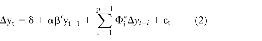
where
Model and implementation details
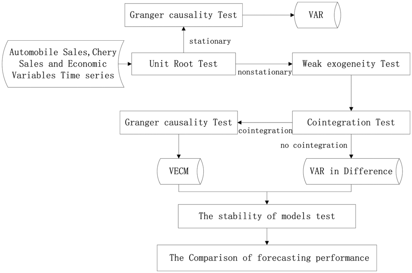
The framework of Chinese automobile sales forecasting model is shown in Figure 3. In econometric model, the stationarity of the time series should be discussed before analyzing the time series. First, the unit root test is carried out. If the test result is stationary, VAR is imported. Otherwise, VAR is established in the form of difference. Furthermore, weak exogenous is tested, which solve the problem of over-parameterization and determine the structural relationship between endogenous variables. Through cointegration test, it is analyzed whether there is a long-term equilibrium relationship between endogenous variables. Then, the Granger-causality test is adopted to determine whether the relationship is causal. If there are a cointegration relationship and a causal relationship among endogenous variables, the VECM can be imported to forecast.
The framework of Chinese automobile sales forecasting model.
Unit root test
The stationarity of time series requires to be examined by unit root test. There are a lot of types in the unit root test, such as Dickey–Fuller (DF) test, augmented Dickey–Fuller (ADF) test, and Phillips–Perron (PP) test. As a natural extension of the DF, ADF is used to test the stationarity of sequence.17–19 Selecting the lag value is also important for the ADF. Akaike information criteria (AIC) and Schwarz criterion (SC) are commonly used to select the number of lag to determine p value in this article.20–22 The principle of the method determining the p value tries to make sure that the values of AIC and SC are minimal. The null hypothesis of the ADF is that there is one unit root at least, and the alternative hypothesis is that the sequence does not have a unit root. Table 2 lists the ADF test statistics of the original and differenced variables for the unit root. The test results showed that the null hypothesis of unit root cannot be rejected for original variables. For the first differenced variables, the ADF test statistics reject the null hypothesis of unit root. Based on the empirical results, all original variables are treated as non-stationary I(1) series, complying with the prerequisite for modeling VECM.
ADF unit root test of original and differenced variables.

ADF: augmented Dickey–Fuller.
Δ is the difference operator; C, T, and K represent the constant, trend, and lag in test type, respectively. N refers to the type that does not include C or T, and the lag items are added to make the residual white noise.
Weak exogeneity test
It is required to model VAR before weak exogeneity test, which differs from Granger-causality test before modeling. All variables in different form are imported into a VAR. Most important in this process is to select the lag order p. When selecting p, both the enough number of lag and enough freedom should be met. In addition to AIC and SC, the lag length criterion should also include the continuous corrected likelihood regression (LR) test statistics, the Hannan–Quinn (HQ) criterion, and the final prediction error (FPE) criterion. The result of lag length selection is given in Table 3. All criteria select a lag length of two, except the SC and HQ. Therefore, lag 2 is selected for the Granger-causality test.
Lag length selection criteria.
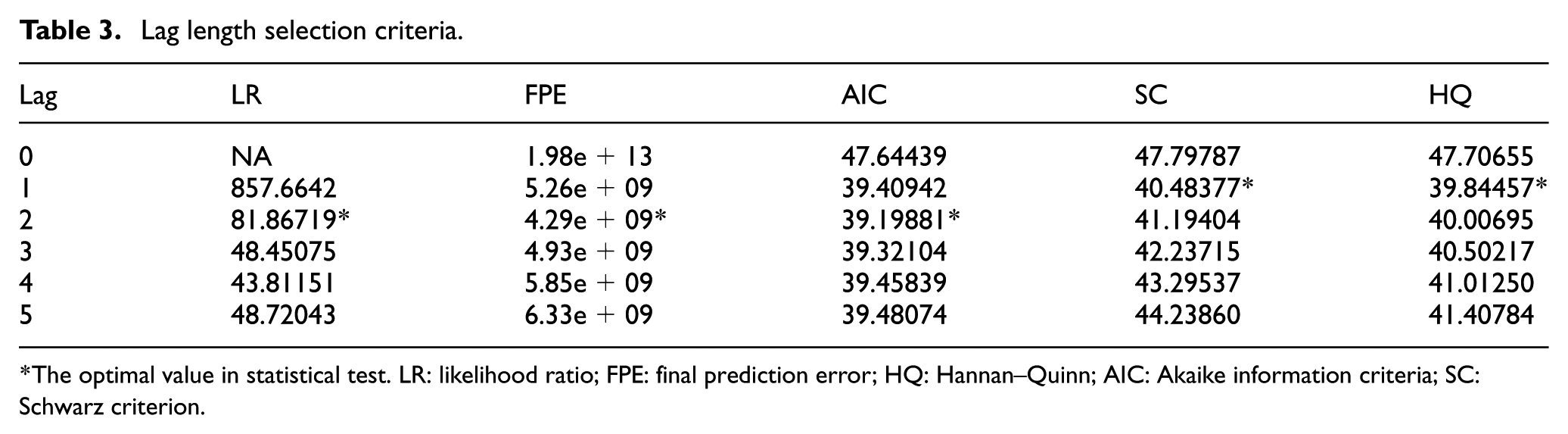
The optimal value in statistical test. LR: likelihood ratio; FPE: final prediction error; HQ: Hannan–Quinn; AIC: Akaike information criteria; SC: Schwarz criterion.
To avert the sensitivity of exogenous variables on the model norm, weak exogenous test is used to differentiate between the internal and external properties of variables.23–26 The purpose of weak exogeneity test is to identify the weak exogeneity impact among each variable. Besides, weak exogeneity test can deal with the question of over-parameterization in VAR and VECM, with which the model equations containing some exogenous variables can be simplified. At the significant level of 5%, the null hypothesis is rejected, that is, the existence of structural relationship is received. Table 4 lists the results of weak exogeneity test, and the relationship of variables in weak exogeneity test is shown in Figure 4. The result shows that except for log(X2) and log(X3) in this study, there are some structural relationships among variables. In subsequent analysis, log(X2) and log(X3), therefore, are treated as exogenous variables.
Weak exogeneity tests.
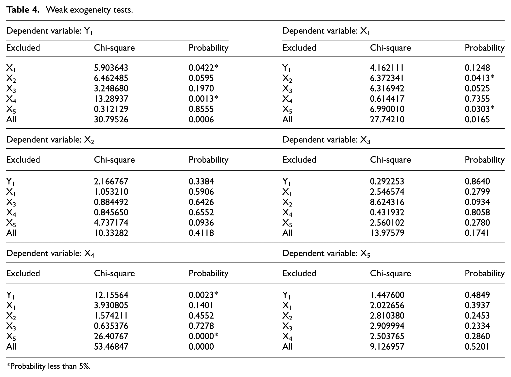
Probability less than 5%.

The relationship of variables in weak exogeneity test.
Cointegration test
Engle and Granger proposed that VECM can be modeled only if a long-run equilibrium relationship exists among variables, so it requires cointegration test before modeling.
27
In the light of the principle of unit root test, all variables related to the model are viewed as I(1) series in the subsequent analysis, so the cointegration can be tested on variables directly. Johansen28,29 test has been applied extensively in cointegration test, and it lists all the cointegration relationships among variables, and the test function of Johansen test is more steady than the Engle and Granger test. Johansen test is a cyclic process in fact. The test starts with the hypothesis of
Johansen’s cointegration trace tests.
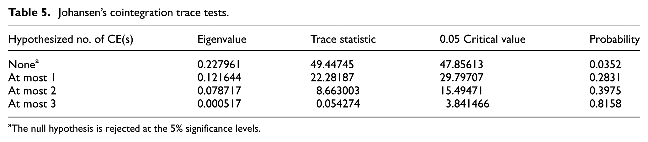
The null hypothesis is rejected at the 5% significance levels.
Johansen’s cointegration max-eigen tests.

The null hypothesis is rejected at the 5% significance levels.
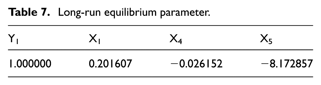
There is one cointegration vector among four variables according to the test results. The standardized long-run equilibrium parameter for log(Y1) is shown in Table 7. So, the long-run relationship among four variables is given as follows

Long-run equilibrium parameter.
Granger-causality test
Granger-causality test can decide whether the relationships among variables are causal, and it can also distinguish exogenous variables from all variables. When predicting Y, if the predicting result based on the historical data of both X and Y are better than that only based on the historical data of Y, then there is the causal relationship between economic variables X and Y. In the case of no-cointegration relationship among variables in the model, this theory can be tested for a judgment of endogenous and exogenous variables in the VAR and VECM. F-Statistic is used to do Granger-causality test in this article. Table 8 shows the results of Granger-causality tests. If p value is less than 5%, the null hypothesis must be accepted, that is, there is a causal relationship among tested variables. Otherwise, the null hypothesis is rejected. The relationship of variables in Granger-causality test is shown in Figure 5, which illustrates that there are causal relationships among variables except log(X2) and log(X3). The result of weak exogeneity is consistent with Granger-causality test. So, these two economic variables must be considered as exogenous variables.
Granger-causality test.
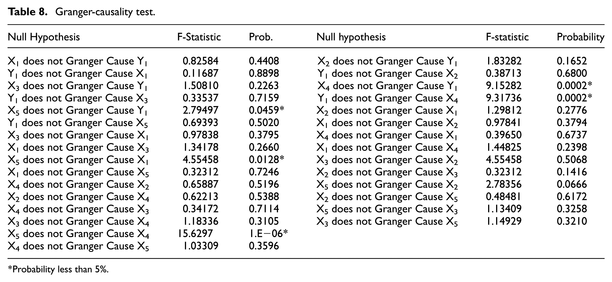
Probability less than 5%.

The relationship of variables in Granger-causality test.
The evaluation of forecasting performance
The establishment of the forecasting model
The cointegration relationship among Chinese automobile sales, Chery sales, and economic variables is tested by the cointegration test. When the VAR model is applied, the error correction vector, therefore, should be added into model. In other words, the residuals of each variable are added into the estimation. 16 The VECM can be derived from the auto-regressive distribution hysteresis model, and each equation in the VAR is an auto-regressive distribution hysteresis model. Thus, the VECM can be considered as the VAR with cointegration constraints.
Based on these theories, the VAR in difference form and VECM are established by endogenous variables and the results are as follows:
VAR:

VECM:

The stability of the model test
It is necessary to test the stationary of the VAR and VECM of automobile sales. If the estimated moduli of roots of VAR and VECM are less than 1, that is to say, they lie in the unit circle, the VAR and VECM are said to be stationary. There are K × P roots in VAR, in which the number of endogenous variables is K and the number of optimal lag of VAR in difference is P. There are K × P roots in VECM, in which the number of endogenous variables is K and the number of optimal lag of VAR is P. The stationarity tests of VAR and VECM are given in Tables 9 and 10, respectively.
The stationarity test of VAR.

The stationarity test of VECM.
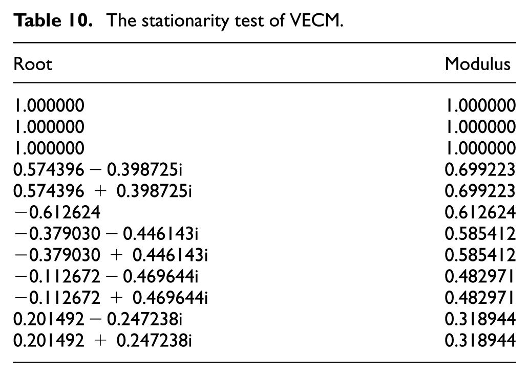
As shown in Tables 9 and 10, the moduli of roots of VAR and VECM lie in the unit circle. This indicates the VAR and VECM previously established in this paper are steady. Thus, the forecasting results of the VECM and VAR of automobile sales are reliable. There are r cointegration relationship in VECM and modulus of roots of k − r equals to 1.
Forecasting performance and comparison
In order to show the forecasting performance, VAR and ARMA are used to compare with VECM in this article. Both the root mean square error (RMSE) and mean absolute percentage error (MAPE) are computed for the comparison of forecasting accuracy. The results are shown in Table 11. The comparison of 12-period automobile sales forecasting values and actual value in 2016 is shown in Figure 6. Compared with the VAR and ARMA, RMSE (0.1243) and MAPE (10.2015) by VECM for 12-period forecasting are minimal. That means prediction accuracy by VECM is the best.
12-period forecasting comparison (with ARMA and VAR models).

Optimal results. RMSE: root mean square error; MAPE: mean absolute percentage error; ARMA: auto-regressive moving average; VECM: vector error correction model; VAR: vector auto-regression.

The comparison of 12-period automobile sales in 2016.
When Chery sales are used to forecast automobile sales as the endogenous variables, the result shows that the VECM outperforms VAR and ARMA. Moreover, comparison between ignoring and considering the impact of Chery sales is shown in Figure 7. The results show that the prediction accuracy of considering the impact of Chery sales is relatively superior, which means that the fluctuation trends of Chinese automobile sales and Chery sales are closely linked.
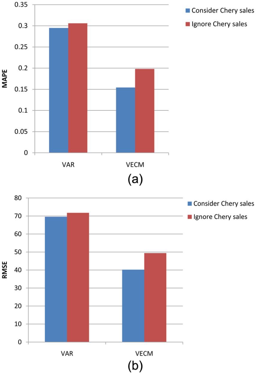
Comparison between ignoring and considering the impact of Chery sales: (a) MAPE comparison and (b) RMSE comparison.
Conclusion
In this article, in order to analyze the intrinsic correlation among Chinese automobile sales, Chery sales, and economic variables, an econometric model is proposed. The monthly data from 2007 to 2016 are used for empirical analysis. The conclusions are as follows:
There are the dynamic connections among Chinese automobile sales, typical domestic brand automobile sales, and economic variables. The forecasting method based on econometric model is effective. The unit root test results indicate that all variables in the dataset are non-stationary and the variables in first difference are stationary. For the weak exogeneity and Granger-causality tests, two conclusions are consistent that the CCI and CPI are exogenous variables. The long-term equilibrium relationship among Chinese automobile sales, Chery sales, gasoline price, and steel production is validated by Johansen cointegration test. Based on long-term equilibrium relationship, VECM is established to reflect the dynamic process of adjusting from short-term departure to the long-term equilibrium among the variables, and the dynamic evolution among variables is clearly defined. This article analyzes the relationship between automobile sales and variables and improves the forecasting accuracy of automobile sales by introducing VECM.
Compared with VAR and ARMA in the long-term forecasting results, VECM can improve the prediction accuracy in terms of RMSE and MAPE. According to the comparison between ignoring and considering the impact of Chery sales, the prediction accuracy of considering the impact of Chery sales is relatively superior, which succeeded in improving the forecasting accuracy of automobile sales even further. So, the fluctuation trends of Chinese automobile sales and typical domestic brand automobile sales are closely linked.
Although the method adopted and the results are satisfactory, the number of economic variables used is still limited due to the difficulty of collecting the relevant monthly data. Therefore, the future work could try to test the relationship between automobile sales with more economic indicators, find out more endogenous variables, and improve the forecasting model.
Footnotes
Handling Editor: Gang Chen
Declaration of conflicting interests
The author(s) declared no potential conflicts of interest with respect to the research, authorship, and/or publication of this article.
Funding
The author(s) disclosed receipt of the following financial support for the research, authorship, and/or publication of this article: This work is partially supported by Liaoning province PhD startup Fund Project (20170520365) and Humanity and Social Science Youth foundation of Ministry of Education of China (13YJCZH042).