Sage Journals: Discover world-class research

Abstract

Blade tip timing is a contactless method used to monitor the vibration of blades in rotating machinery. Blade vibration and clearance are important diagnostic features for condition monitoring, including the detection of blade cracks. Eddy current sensors are a practical choice for blade tip timing and have been used extensively. As the data requirements from the timing measurement become more stringent and the systems become more complicated, including the use of multiple sensors, the ability to fully understand and optimize the measurement system becomes more important. This requires detailed modeling of eddy current sensors in the blade tip timing application; the current approaches often rely on experimental trials. Existing simulations for eddy current sensors have not considered the particular case of a blade rotating past the sensor. Hence, the novel aspect of this article is the development of a detailed quasi-static finite element model of the electro-magnetic field to simulate the integrated measured output of the sensor. This model is demonstrated by simulating the effect of tip clearance, blade geometry, and blade velocity on the output of the eddy current sensor. This allows an understanding of the sources of error in the blade time of arrival estimate and hence insight into the accuracy of the blade vibration measurement.

Keywords

Eddy current sensor blade tip timing electro-magnetic field quasi-static finite element model

Introduction

In recent years, the identification of damage in rotating blades has been of great importance. Contact measurement and data processing techniques have been proposed to monitor the vibration of blades in the rotating frame. One of the basic contact methods is the strain-gauge system which appeared in the 1960s.¹ This approach involves mechanically attaching transducers to the selected blades to provide vibration measurements. This method has several shortcomings; it is time consuming, is fragile with respect to the ability to withstand the gas turbine environment, and is restricted to only few blades of the turbines. Therefore, many investigators have considered contactless diagnostic systems to monitor blade vibrations in the rotating frame due to the non-intrusive and easy installation of sensors which allows prompt detection of potential cracks. One of the well-known methods is the so-called blade tip-timing (BTT) method, named also as the Non-Contact Stress Measurement System (NSMS). The BTT method is based on analyzing the time histories of single blades with respect to the position of stationary sensors, called the blade time of arrival (ToA). This is compared to the speed of revolution which leads to the measurement of vibrations since the blade ToA is influenced directly by the vibration amplitude and frequency. In addition to the vibration measurement, further diagnostics to detect cracks can be performed based on the measurement of blade tip clearance (BTC), which is the distance separating the blade tip to the engine casing. These measurements can also be provided by the blade-tip sensors.

During the early 1970s, the first non-contact measurement was introduced by Zablotskiy and colleagues^2,3 based on their own device to measure vibration called ELURA. Heath⁴ and Heath and Imregun⁵ extended the Zablotskiy–Korostelev technique by providing a rigorous and enhanced formulation to derive the blade arrival times using optical laser probes. Several sensing technologies have been proposed to monitor blade positions in turbomachinery relying on capacitance, inductance, optics, microwaves, and eddy currents. Von Flotow et al.⁶ summarized a variety of vibration blade monitoring technologies, and they pointed out the need to distinguish between the effect of cracks and any other source of damage (e.g. thermal expansion or centrifugal force) on the blade lengthening measurements. In the last decade, Zielinski and Ziller^7–9 described several developments in non-contact blade vibration measurement based on crack detection techniques by illustrating various experimental applications. Blade vibration measurement using capacitance probes has also been investigated by Lawson and Ivey^10,11 due to the dual potential of this type of probe to provide measurement for both tip clearance and tip timing. Due to its low cost and temperature resistivity, a single optical probe was used by Kempe et al.¹² in a measurement system to present proof-of-principle measurements for a novel tip-clearance measurement technique with high spatial and temporal resolution. In addition, an improved capacitance probe has been used extensively by major European gas turbine manufacturers for high-temperature turbine applications and was described by Sheard.¹³ He presented BTC measurement techniques and laboratory experiments to explore probe reliability at high temperature. Procházka and Vaněk¹⁴ illustrated a contactless diagnostic method to identify a steam turbine blade’s strain, vibration, and damage. They suggested an improved tip-timing method based on the utilization of a diagnostic system (VDS-UT) and new magneto-resistive sensors. Woike et al.^15,16 outlined key results and contributions from three different structural health monitoring approaches using BTC sensors. Garcia et al.^17,18 tried to overcome several traditional shortcomings of capacitive, inductive, and discharging probes in measuring the blade tip timing and clearance in turbines. Consequently, they proposed a probe based on a trifurcated bundle of optical fibers mounted on the turbine casing. Based on their approach, the tip clearance measurements and the blade tip timing were simultaneously measured, leading to lower cost and time requirements. More recently, Guo et al.¹⁹ established a model of the BTT signal from a fiber bundle sensor. Based on simulation results, they successfully eliminated the measurement error caused by this change of the clearance between the blade and the sensor using a variable gain amplifier to amplify the signals to a similar level.

Many researchers have explored the potential of eddy current sensors (ECS) to assess the health of an engine without any need for direct access to the blade (e.g. the possibility to monitor through the casing). ECS are also insensitive to the presence of any type of contaminant (e.g. fluid or high temperature). Both tip timing and tip clearance of each blade could be measured by these sensors in real time and at high resolution. However, some limitations such as case thickness or material could be a major obstacle in monitoring the system. Garcia-Martin et al.²⁰ provided a summary of the basics and important variables of eddy current testing. They reviewed the state of the art of eddy current testing for crack detection in a variety of electrical conductive materials. In terms of experimental studies investigating the eddy current assessment of rotating systems, Lackner²¹ assembled a test rig of three spinning test blades to test the ability of ECS in a simulated gas turbine environment. Compared to strain gauge data extracted from the test rig, he showed that ECS could mitigate the drawbacks of other types of sensors, such as optical or capacitive sensors. Rahman and Marklein²² provided a numerical model of ECS for an in-line assessment of hot wire steel. They used a different numerical method with the aim to model a nondestructive testing system. The arrival times of a rotor blade based on ECS were measured by Chana and Cardwell²³ in various engine trials to evaluate the ability of these sensors to detect pre-existing damage and to capture dynamic foreign object damage events. They demonstrated that high-quality tip timing data could be obtained from the experiments. Similarly, Cardwell et al.²⁴ pursued the prospect of using ECS for the measurement of blade tip timing in rotor machinery. They developed an improved ECS system through laboratory tests to measure rotor blade arrival times. In addition, Chana et al.²⁵ evaluated the ability of an ECS and Reasoner software system to isolate a crack propagated in a cyclic engine and to predict its remaining useful life. More recently, Mandache et al.²⁶ developed pulsed eddy current technology to monitor the health of the engine through its casing based on blade tip displacement. Using a simple 3-blade assembly, a “through the casing” transmit/receive pulsed eddy current probe was employed to investigate variations in BTC, inter-blade spacing, and blade twist/angle. An improved blade tip timing method was proposed by Liu and Jiang.²⁷ They introduced an ECS to detect the torsional vibrations of the rotor. Haase and Haase²⁸ used through-the-case ECS to present advances in tip clearance measurement systems for turbine engines. Using a combination of ECS and optical sensors, Guru et al.²⁹ instrumented a low pressure turbine stage of a developmental aero engine to monitor blade vibrations during engine tests. In terms of analytical modeling of eddy current field, Karakoc et al.^30,31 derived an analytical model of an eddy current brake (ECB) under time-varying magnetic fields. They investigated the effect of the time-varying field on the braking torque. To predict small fatigue cracks, Rosell and Persson³² performed an eddy current contactless inspection based on finite element model and experiments.

The past investigations using eddy current testing in blade tip timing of rotating blades have been predominantly experimental and have ignored the accuracy of the timing measurement, which depends on the blade deformation and clearance between the blade and the sensor. They also ignored the geometry effects on the measurement and have just concentrated on extracting response frequencies. As the requirements from the BTT system becomes more stringent, for example using multiple sensors to extract bending and torsional responses from blades with a complex geometry, the optimization of the measurement system cannot be undertaken experimentally. Further development of BTT systems therefore requires detailed models of both the sensor and the rotating bladed disk. Hence, for the first time, quasi-static 2D and 3D finite element models of the electro-magnetic field are developed in this article to simulate the integrated measured output and to investigate the effects of blade tip geometry, clearance, and rotational speed on the ECS output. A rotating blade with simple geometry, passing a single eddy current sensor, is used to understand the modeling difficulties and requirements. One important example of these difficulties, highlighted in this article, is the more stringent requirements on the finite element mesh at the interface between the rotating and stationary parts of the model. The simulated sensor output has the same form as outputs obtained from the many experiments in the literature.

This article is arranged as follows. The principle of eddy current sensor in monitoring a moving target is described in section “Mechanics of ECS in monitoring a moving target.” The governing equations for modeling a moving target in an electro-magnetic field are presented in section “Governing equations for modeling of ECS.” A numerical method for blade tip timing using an eddy current sensor is described in section “The simulation of blade tip timing using an ECS,” where mesh details and boundary conditions are presented. Finally, section “Simulations for the moving bladed disk and ECS” contains a parametric study and concluding remarks.

Mechanics of ECS in monitoring a moving target

In this section, the concept of eddy current monitoring is described. Eddy currents are generated when a conductive material moves through a permanent magnetic field, or when an alternating magnetic field acts on a conductive target. These cases correspond to a passive ECS and an active ECS, and both types of sensors have been used for BTT measurements. In the case of an active ECS, the operating principles are understood as follows.²⁰

An alternating current in the coil of the ECS generates a time-varying magnetic field formed around the coil. If an electrically conducting target is moving past, the primary magnetic field penetrates the moving object causing a variation of the magnetic flux through it. Following Faraday’s law of induction, this induces a flow of electric current, named the eddy current. The induced currents in the target generate a secondary magnetic field that acts against the primary magnetic field as shown in Figure 1. Therefore, a change in the impedance of the coil is captured by the sensor. Measuring the change in the coil impedance is related to the gap between the sensor and the target, and commercial sensors are calibrated so that the sensor output gives the relative displacement. A passive ECS works in a similar way, except that a permanent magnetic field is generated, and the motion of the conductive blade through the magnetic field generates eddy currents. These eddy currents generate the secondary magnetic field, which is measured by the sensor. The magnetic field needs to vary to generate an output in the sensor coil and hence a passive ECS essentially measures velocity. Thus, a passive ECS is not used as a displacement sensor, but does work well for blade tip timing where the blade is always moving past the sensor. The model in this article considers a passive ECS.

Figure 1.

The eddy current sensor concept.

Governing equations for modeling of ECS

In this section, the model of an eddy current sensor for a moving target is developed. For a moving target, Maxwell’s equations (equations (1)–(4)) along with constitutive relations (equations (5) and (6)) and the magnetic and electric material properties of the target are used to describe the electro-magnetic field in terms of sources as^31,32

\nabla \times H = J + \frac{\partial D}{\partial t}

(1)

\nabla \times E = - \frac{\partial B}{\partial t}

(2)

\nabla \cdot D = ρ

(3)

\nabla \cdot B = 0

(4)

D = ε E

(5)

B = μ H

(6)

where $H$ is the magnetic field strength, $B$ is the magnetic flux density, $E$ is the electric field, $D$ is the displacement flux density, $J$ is the current density, $ρ$ is the charge density, $μ$ is the magnetic permeability, and $ε$ is the electric permittivity of the medium.

In the particular problem of an eddy current sensor, the electric current generated is composed of two parts

J = J_{t} + J_{s}

(7)

where $J_{t}$ is the current density induced in the electro-conductive target neighbor with the coil sensor and $J_{s}$ is the current density in the coil region of the sensor generated by the voltage supply in this coil. Following Ohm’s law for a moving conductor, along with the presence of the magnetic field, the eddy current generated in the target is defined as

J_{t} = σ (E + v \times B)

(8)

where $v$ is the velocity of the target and $σ$ is the conductivity of the target’s medium.

Satisfying two of Maxwell’s equations, equations (2) and (4), the magnetic vector potential $A$ and the scalar potential $φ$ are defined as

E = - \nabla φ - \frac{\partial A}{\partial t}

(9)

B = \nabla \times A

(10)

Since the eddy current problem is a magneto-quasi-static problem,³⁴ the displacement current can be ignored, that is, $\partial D / \partial t \approx 0$ . Therefore, substituting equations (6)–(10) into equation (1) yields

\nabla \times B = μ J + σ μ (E + v \times B)

(11)

By rearranging the terms in equation (11) and replacing the electric field and magnetic flux density by their expressions in equations (9) and (10), we obtain, in terms of $A$ and $φ$ , the following magnetic governing equation

\nabla \times (\nabla \times A) - μ σ (- \nabla φ - \frac{\partial A}{\partial t} + v \times (\nabla \times A)) = μ J_{s}

(12)

The simulation of blade tip timing using an ECS

In this section, a simulation of the distribution of an eddy current generated by an ECS in a simple rotating bladed disk (e.g. blisk) is described as a time-dependent electro-magnetic 3D and 2D problem on a cross section through the model. A simple model was considered in this study to investigate the effects of gross changes in geometry and highlights the effects of geometry parameters on the BTT measurements. This presents a first step toward realistic geometries where it is complicated to change parameters easily. To achieve this task, a commercial FEA software package, COMSOL Multiphysics®,³⁵ was used.

Geometry details of the two-dimensional and three-dimensional model

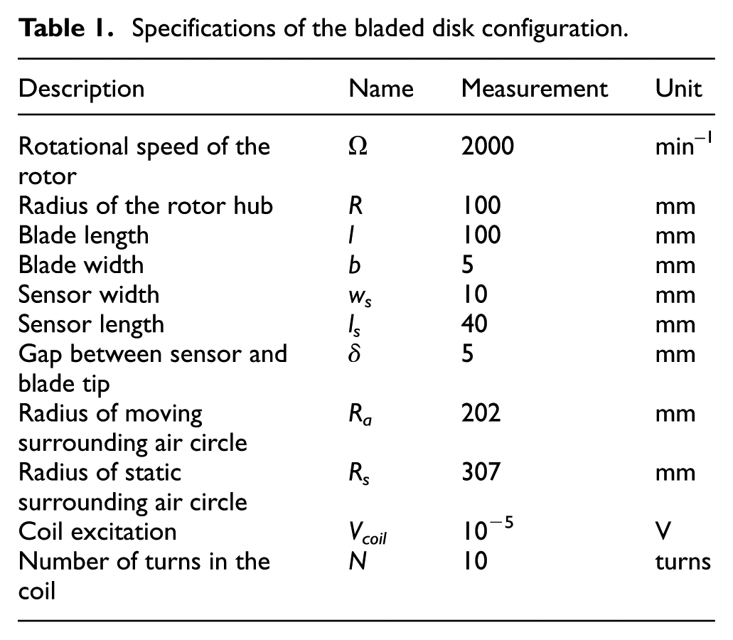
The two-dimensional (2D) and three-dimensional (3D) geometry of the model were generated based on the design parameters given in Table 1. As shown in Figure 2, the bladed disk (or blisk) is composed of a disk with radius R and four simple rectangular blades of length l and width b. A rectangular surface of length l_s and width w_s in the 2D geometry and a corresponding cuboid volume in the 3D geometry were considered to simulate an eddy current sensor separated by an air gap δ from the blade tips as shown in Figure 3(b).

Table 1.

Specifications of the bladed disk configuration.

Description	Name	Measurement	Unit
Rotational speed of the rotor	Ω	2000	min^–1
Radius of the rotor hub	R	100	mm
Blade length	l	100	mm
Blade width	b	5	mm
Sensor width	w_s	10	mm
Sensor length	l_s	40	mm
Gap between sensor and blade tip	δ	5	mm
Radius of moving surrounding air circle	R_a	202	mm
Radius of static surrounding air circle	R_s	307	mm
Coil excitation	V_coil	10⁻⁵	V
Number of turns in the coil	N	10	turns

Figure 2.

The model geometry: (a) 2D model and (b) 3D model.

Figure 3.

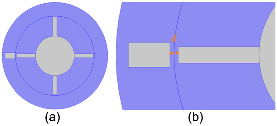
The geometry of the (a) surrounding air of the 2D model (b) air gap.

The essential part of the problem is the definition of the rotating and non-rotating regions of the model as separate geometric objects. Therefore, to discretize the 2D and the 3D domain of the model, a steady rotation of the rotor is imposed.

The surrounding air is added to the geometry as circular surfaces (a cylindrical volume for the 3D domain) which enclose the rotating and non-rotating parts of the model, respectively (the surrounding air is highlighted in Figures 3 and 4).

Figure 4.

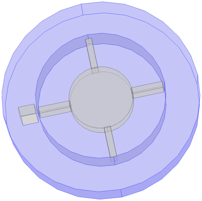
The geometry of the surrounding air of the 3D model.

The geometry is cut along the air gap (shown in Figure 3(b)) into two adjacent parts: one including the fixed part of the model which consists of the sensor and some surrounding air, and the other containing the moving part composed of the blisk and some surrounding air, as shown in Figure 5. The moving and static regions are then coupled using the ‘Form Assembly’ option in COMSOL, which allows a controlled discontinuity in the scalar magnetic potential at the interface.

Figure 5.

The geometry of the moving and static parts: (a) 2D model and (b) 3D model.

Boundary conditions and physics applied

After creating the different regions of the model, the boundary conditions at the interface are generated. At the interface between the rotating part and the static part, the continuity of the magnetic scalar potential must be enforced in the global fixed coordinate system. Also, a quasi-static approximation is applied where the displacement current density is ignored. Based on this approximation, the total current in the model arises from the eddy currents induced in the moving blades and those externally applied through the permanent field generated by the eddy current sensor.

The COMSOL software uses two approaches to solve Maxwell’s equation, using either the magnetic vector potential or the magnetic scalar potential. The magnetic vector potential allows for current-carrying domains and hence is used to solve coil and conducting domains. It can be modeled with Ampere’s law feature in the software and is the most general formulation. On the other hand, the magnetic scalar potential introduces fewer degrees of freedom and ensures a better accuracy of the magnetic flux density coupling when it is used to enforce the continuity of two sectors and therefore it is used to solve air regions. This formulation is included as the Magnetic Flux Conservation feature in the software. In the 2D model, the formulation of Ampere’s law is applied in all domains. However, in the 3D model, the two formulations are combined and referred as a mixed formulation, where the conductive part of the rotating part (e.g. the blisk) is modeled using Ampere’s law feature, whereas the nonconductive part (i.e. the surrounding air, both rotating and static) are modeled using Magnetic Flux Conservation feature for the scalar magnetic potential based on the assumption that the magnetic field is curl free in the no-current region. This gives a significant decrease in the computational time and increases accuracy of the pair coupling given by the scalar formulation at the common boundary that separates the rotating part from the static part. Finally, the blisk and sensor are assumed to be solid aluminum. The eddy current sensor is modeled using the COMSOL interface called Coil Domain which models a conductive domain subject to a lumped excitation, such as voltage, current, or power. For better convergence, a closed curve in the scalar potential region (e.g. air region) should not contain a magnetic vector potential region that is carrying a current (e.g. coil region). Therefore, an additional cuboid region modeled with Ampere’s law was added to surround the sensor (as shown in Figure 6) to enhance the electro-magnetic model convergence. In addition, the coil voltage was ramped up from 0 to 1 V over 0.25 s (approximately eight rotations of the blisk), so that excessive transients are not excited. The rotational speed is assumed to equal Ω = 2000 r/min. The model is then simulated in the time domain for 0.3 s.

Figure 6.

Cuboid region modeled with Ampere’s law.

Mesh details of the 2D and 3D model

In terms of meshing, triangular elements were used in the discretization of the 2D model while in the 3D model, tetrahedral elements were used, as shown in Figures 7 and 8, respectively.

Figure 7.

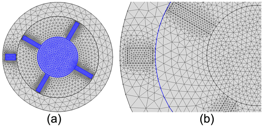
Mesh details of the 2D model: (a) bladed disk and sensor and (b) the cut boundary.

Figure 8.

Mesh details of the 3D model: (a) bladed disk and sensor and (b) the cut boundary.

A refinement across the entire volume of the blades is performed since the eddy currents are at their highest density in the blades. In addition, due to the creation of an assembly, the two parts (rotating and static) are meshed separately, as shown in Figures 7 and 8 by the distinct positions of the mesh nodes on each side of the interface. A fine mesh is used on the Continuity Boundary, in particular the rotating part of the Boundary is meshed more finely than the stationary part of the Boundary in order to make the continuity applied at this boundary more accurate and the model therefore more stable. These two parts with the corresponding meshes always stay in contact at the cut boundary for the two models, as highlighted in blue in Figures 7(b) and 8(b). The moving mesh approach is supported by COMSOL.

Since the mesh density varies from one domain to the other through the geometry of the model, a mesh refinement study has been performed to optimize the computation time and obtain converged results. Regarding the 2D model, it was noticed that the moving surrounding air domain (the highlighted surface in Figure 9) has the most effect on the convergence of the results and therefore the mesh of that domain was refined by decreasing the mesh element size and therefore increasing the number of elements, as shown in Figure 9. The total number of elements used was 23,920. Figure 10 shows the measured sensor signal corresponding to the mesh shown in Figure 9. In Figure 10(a), corresponding to the mesh shown in Figure 9(a) with 12,638 elements, the high frequency noise is due to nodes passing at the interface. Increasing the number of elements to 23,920, which corresponds to the mesh in Figure 9(b), this high frequency noise decreases, as shown in Figure 10(b).

Figure 9.

Mesh refinement of moving surrounding air domain: (a) 12,638 elements and (b) 23,920 elements.

Figure 10.

Effect of mesh refinement on the coil current output corresponding to different meshes: (a) 12,638 elements (Figure 9(a)) and (b) 23,920 elements (Figure 9(b)).

Simulations for the moving bladed disk and ECS

All results shown in this section were generated by the COMSOL software for the fixed geometric parameters in Table 1, apart from the parameter that is explicitly varied. Figure 11 shows the comparison of the coil current output corresponding to the 2D and 3D models, generated for the same geometric parameters. The small difference between the two models is probably due to the effect of the thickness of the disk in the 3D model. Overall, there is an excellent agreement between the two models, giving confidence in the equivalence of the 2D and 3D models in this configuration. Since the 3D models require significant computational resources (around 12 h per simulation), the following results are obtained from the 2D model.

Figure 11.

Comparison of the coil current output for the 2D and 3D models.

Figure 12 shows the surface plot of the norm of the magnetic flux density at the initial time, t = 0 s. The magnetic vector potential is also shown by magnetic flux lines induced thorough the plane of the bladed disk. There is no variation or effect on the magnetic flux lines since the blades are still static and the electro-magnetic field is continuous across the surrounding air, since a homogeneous material is assumed.

Figure 12.

Magnetic flux density norm (surface) and magnetic vector potential Z-components (contour) at t = 0 s: (a) whole model and (b) a locally enlarged region.

At t = 0.0025 s, one of the blades passes the ECS, and Figure 13 shows the variation in the induced magnetic flux lines. This variation is due to the interference between the primary magnetic field generated by the ECS and the secondary magnetic field generated by the blades moving past the sensor. This agrees with the concept of ECS described in section “Mechanics of ECS in monitoring a moving target.”

Figure 13.

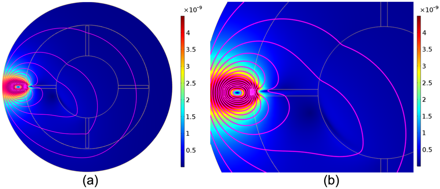
Magnetic flux density norm (surface) and magnetic vector potential Z-components (contour) at t = 0.0025 s: (a) whole model and (b) a locally enlarged region.

Figure 14 shows the corresponding coil current output captured by the sensor as a blade passes by. A peak in the signal is obtained every time a conducting blade enters the field of the sensor, which alters the magnetic field through the induced eddy currents in the blades. Figure 14(b) shows the shape of a single peak and includes a line corresponding to the initial coil current generated by the sensor. This gives a reference to determine when the blade is positioned at the middle of the sensor, which gives information about the time of arrival of the blade at the sensor.

Figure 14.

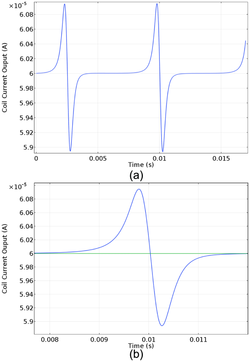
The coil current output: (a) several blade passes and (b) a single blade passing.

Figure 15 shows the effect of the variation of the width of the moving blades. By increasing the width of the blade, the amplitude of the sensor signal increases. Also, as expected, we notice a translation of the time corresponding to the peak of the signal since the width is increasing. This is due to the large disturbance caused by the larger blade width in the magnetic field.

Figure 15.

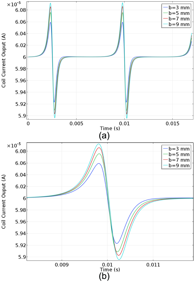
The coil current output with time for different blade widths: (a) several blade passes and (b) a single blade passing.

Figure 16 shows the effect of the blade length variation on the induced voltage in the sensor. Increasing the blade length increases the amplitude of the sensor signal because the tip velocity increases.

Figure 16.

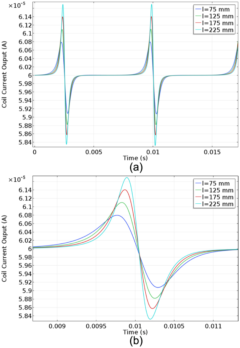
The coil current output with time for different blade lengths: (a) several blade passes and (b) a single blade passing.

This effect is further clarified by Figure 17, which shows the magnetic vector potential over the geometry of the model, corresponding to the shortest and longest blades, among the different lengths used in Figure 16. The discrepancy in the magnetic vector potential is more pronounced for the longer blade (Figure 17(b)) than for the shorter blade (Figure 17(a)) and causes the higher amplitude. Also, the signal corresponding to the shorter blade (i.e. the blue line in Figure 16(a)) behaves slightly differently to the other curves between the two peaks. This is due to the impact of the rotor disk on the induced eddy currents.

Figure 17.

Magnetic flux density norm (surface) and magnetic vector potential Z-components (contour) at t = 0.0025 s: (a) blade length l = 75 mm and (b) blade length l = 225 mm.

Figure 18 shows that the amplitude of the sensor signal increases with increasing radius of the disk. Since the rotational speed is constant, increasing the radius of the disk will increase the tip radius, and hence the speed the blade passes the sensor. Hence, the amplitude of the peaks in the induced voltage increases with the disk radius.

Figure 18.

The coil current output with time for different disk radius: (a) several blade passes and (b) a single blade passing.

Figure 19 shows the effect of the variation of the gap (i.e. the distance separating the blade tip and the surface of the sensor during the rotation of the bladed disk) on the sensor output. There is a clear decrease in the signal amplitude with increasing gap between the sensor and the blade tip. This shows the sensitivity of the ECS to small distance variations.

Figure 19.

The coil current output with time for different blade gaps: (a) several blade passes and (b) a single blade passing.

Finally, Figure 20(a) shows the effect of the rotational velocity of the bladed disk on the sensor voltage. This figure is difficult to interpret since there is no reference to the blade position. The output current curves should be shifted so that the blade passes the sensor at the same time, as shown in Figure 20(b). The amplitude of the signal tends to increase with the rotational speed. This sensitivity shows that the speed of the target moving past the sensor could be a source of error in the BTT measurement.

Figure 20.

The coil current output with time for different rotational speeds: (a) arbitrary phase and (b) after shifting curves to a common phase.

Conclusion

This article has simulated a rotating bladed disk of simple geometry that is surrounded by a casing to which an eddy current sensor has been attached. The aim was to simulate the measurement process used for blade tip timing method using ECS. ECS have been considered in this article due to their robustness in harsh environments. The governing equations modeling the magneto electric field of a moving target have been described for a quasi-static problem. A detailed description of the geometry of the 2D and 3D models was described, together with the meshing difficulties encountered due to the rotation and the physics of the electro-magnetic fields. The simulations gave sensor outputs that correspond to those measured and reported in the literature. The parameter studies showed that the eddy current sensor output is sensitive to the air gap and the sensor location, as well as to the rotational speed of the system. This sensitivity can help to understand the errors that could be introduced due to the inhomogeneities in the blades or the disk and the time of blade passing can be estimated more accurately by taking into consideration these effects. Moreover, this investigation in the sensitivity of the eddy current signal to different model parameters lead to fix strategically these parameters in order to increase damage sensitivity and in terms of experimental work, the voltage picked can be chosen with no influence of the blade. Furthermore, this modeling approach can be utilized to design and optimize blade tip timing systems with multiple sensors, complex geometries, and coupled vibration responses; such studies will be the subject of future research.

Footnotes

Handling Editor: Yaguo Lei

Declaration of conflicting interests

The author(s) declared no potential conflicts of interest with respect to the research, authorship, and/or publication of this article.

Funding

The author(s) disclosed receipt of the following financial support for the research, authorship, and/or publication of this article: The authors gratefully acknowledge the support of the Qatar National Research Fund through grant number NPRP 7-1153-2-432.

References

Fangman

Zastrow

Bobeck

. High-speed-turbocharger blade-vibration measurement. Exp Mech 1967; 7: 19A–21A.

Zablotskiy

Korostelev

. Measurement of resonance vibrations of turbine blades with the ELURA device. Fort Belvoir, VA: Defense Technical Information Center, 1970, p.15.

Zablotskiy

Korostelev

Sviblov

. Contactless measuring of vibrations in the rotor blades of turbines. Lopatochnyye Mashiny I Struynyye Apparaty: Sbornik Statey 1972; 6: 106–121.

Heath

. A study of tip-timing measurement techniques for the determination of bladed-disk vibration characteristics. London: University of London, 1996.

Heath

Imregun

. An improved single-parameter tip-timing method for turbomachinery blade vibration measurements using optical laser probes. Int J Mech Sci 1996; 38: 1047–1058.

Von Flotow

Mercadal

Tappert

. Health monitoring and prognostics of blades and disks with blade tip sensors. In: Proceedings of IEEE aerospace conference, Big Sky, MT, 25 March 2000, pp.433–440. New York: IEEE.

Zielinski

Ziller

. Noncontact vibration measurements on compressor rotor blades. Meas Sci Technol 2000; 11: 847–856.

Zielinski

Ziller

. Noncontact blade vibration measurement system for aero engine application. In: Proceedings of 17th international symposium on air-breathing engines, Munich, 4–9 September 2005, ISABE-2005-1220. AIAA.

Zielinski

Ziller

. Noncontact crack detection on compressor rotor blades to prevent further damage after HCF-failure. In: Proceedings of the NATO AVT-121, symposium, evaluation, control and prevention of high cycle fatigue in gas turbine engines for land, sea and air vehicles, Granada, Spain, 3–7 October 2005, paper no. 19. Research and Technology Organisation.

10.

Lawson

Ivey

. The use of commercially available capacitance tip-clearance probes for tip-timing of aero-engine compressor blades. In: Proceedings of 38th AIAA/ASME/SAE/ASEE joint propulsion conference & exhibit, joint propulsion conferences, Indianapolis, IN, 7–10 July 2002. Reston, VA: AIAA.

11.

Lawson

Ivey

. Turbomachinery blade vibration amplitude measurement through tip timing with capacitance tip clearance probes. Sensors Actuat A: Phys 2005; 118: 14–24.

12.

Kempe

Schlamp

Rösgen

et al . Spatial and temporal high-resolution optical tip-clearance probe for harsh environments. In: 13th international symposium on applications of laser techniques to fluid mechanics, Lisbon, Portugal, 26–29 June 2006. Portugal: Instituto Superior Tcnico.

13.

Sheard

. Blade by blade tip clearance measurement. Int J Rotat Mach 2011; 2011: 516128.

14.

Procházka

Vaněk

. Contactless diagnostics of turbine blade vibration and damage. J Phys Conf Ser 2011; 305: 012116.

15.

Woike

Abdul-Aziz

Oza

et al . New sensors and techniques for the structural health monitoring of propulsion systems. Scientific World Journal 2013; 2013: 596506.

16.

Woike

Abdul-Aziz

Clem

. Structural health monitoring on turbine engines using microwave blade tip clearance sensors. In: Proceedings of smart sensor phenomena, technology, networks, and systems integration, vol 9062, San Diego, CA, 10 April 2014. Bellingham, WA: SPIE.

17.

Garcia

Beloki

Zubia

et al . Turbine-blade tip clearance and tip timing measurements using an optical fiber bundle sensor. In: Proceedings of SPIE 8788, optical measurement systems for industrial inspection (VIII87883H), Munich, 13 May 2013. Bellingham, WA: SPIE.

18.

Garcia

Beloki

Zubia

et al . An optical fiber bundle sensor for tip clearance and tip timing measurements in a turbine rig. Sensors 2013; 13: 7385–7398.

19.

Guo

Duan

Cheng

. Numerical analysis of the blade tip-timing signal of a fiber bundle sensor probe. Opt Eng 2015; 54: 034103.

20.

Garcia-Martin

Gomez-Gil

Vazquez-Sanchez

. Non-destructive techniques based on eddy current testing. Sensors 2011; 11: 2525–2565.

21.

Lackner

. Vibration and crack detection in gas turbine engine compressor blades using eddy current sensors. MSc Thesis, Massachusetts Institute of Technology, Cambridge, MA, 2004.

22.

Rahman

Marklein

. Advanced techniques for modelling and detection of cracks in hot wire steel. In: Proceedings on the 9th European conference on NDT (ECNDT), Berlin, 25–29 September 2006. European Federation for Non-Destructive Testing.

23.

Chana

Cardwell

. The use of eddy current sensor based blade tip timing for FOD detection. In: Proceedings of the ASME turbo expo 2008, Berlin, 9–13 June 2008, pp.169–178. New York: ASME.

24.

Cardwell

Chana

Russhard

. The use of eddy current sensors for the measurement of rotor blade tip timing-sensor development and engine testing. In: Proceedings of the ASME turbo expo 2008, Berlin, 9–13 June 2008, pp.179–189. New York: ASME.

25.

Chana

Cardwell

Gray

. Disk crack detection and prognosis using non contact time of arrival sensors. In: Proceedings of the ASME turbo expo 2011, Vancouver, BC, Canada6–10 June 2011, pp.11–18. New York: ASME.

26.

Mandache

Mcelhinney

Mrad

. Aircraft engine blade tip monitoring using pulsed eddy current technology. In: Proceedings of 4th international symposium on NDT in aerospace(Th-4A3), Augsburg, Germany, 13–14 November 2012. German Society for Non-Destructive Testing.

27.

Liu

Jiang

. Improved blade tip timing in blade vibration monitoring with torsional vibration of the rotor. J Phys Conf Ser 2012; 364: 012136.

28.

Haase

. Advances in through-the-case eddy current sensors. In: Proceedings of aerospace conference, Big Sky, MT, 2–9 March 2013, pp.1–5. New York: IEEE.

29.

Guru

Shylaja

Kumar

. Pre-emptive rotor blade damage identification by blade tip timing method. J Eng Gas Turb Power 2014; 136: 072503.

30.

Karakoc

Park

Suleman

. Improved braking torque generation capacity of an eddy current brake with time varying magnetic fields: a numerical study. Finite Elem Anal Des 2012; 59: 66–75.

31.

Karakoc

Suleman

Park

. Analytical modeling of eddy current brakes with the application of time varying magnetic fields. Appl Math Model 2016; 40: 1168–1179.

32.

Rosell

Persson

. Finite element modelling of closed cracks in eddy current testing. Int J Fatigue 2012; 41: 30–38.

33.

Pohl

Erhard

Montag

. NDT techniques for railroad wheel and gauge corner inspection. NDT&E Int 2004: 37: 89–94.

34.

Haus

Melcher

. Electromagnetic fields and energy. Englewood Cliffs, NJ: Prentice Hall, 1989.

35.

Weststrate

Steinback

Rensing

. COMSOL multiphysics modeling for design optimization of eddy current crack detectors. In: Proceedings of the COMSOL Conference, Boston, MA, 7–9 October 2010. COMSOL, Incorporated.

Simulating eddy current sensor outputs for blade tip timing

Abstract

Keywords

Introduction

Mechanics of ECS in monitoring a moving target

Governing equations for modeling of ECS

The simulation of blade tip timing using an ECS

Geometry details of the two-dimensional and three-dimensional model

Boundary conditions and physics applied

Mesh details of the 2D and 3D model

Simulations for the moving bladed disk and ECS

Conclusion

Footnotes

Declaration of conflicting interests

Funding

References