
Abstract
Supersonic film cooling tangentially ejected through a half Laval nozzle set in a backward-facing slot was numerically simulated to investigate the structures of flowfield and the mechanisms of heat transfer after the slot. In particular, changes in flowfield near the turning point in the cooling effectiveness curve were studied. The turning point is defined by extrapolation of the cooling effectiveness curve using a power-law relationship. The point corresponds to the streamwise position where the hot mainstream is reaching the wall protected by the film coolant and to the disappearance of the unsmooth transition points in streamwise velocity profiles, where the growth rate of velocity in wall normal direction changes gradually from one state to another. The transition of velocity becomes smooth downstream of the turning point. The unsmooth transition point also exists in other profiles of flow parameters, such as the mole fraction of film gas and the total temperature of the fluid, which are indicators of the mixing extent between the mainstream and film coolants. Moreover, the unsmooth transition point is more evident in the film coolant of nitrogen than that of helium due to the slower drop rate of effectiveness in the current configuration of the supersonic film cooling.
Introduction
Film cooling is an effective method used to cool many components exposed to severe heating. Film cooling is typically applied to turbine engines, 1 where cooling air is exhausted through small holes drilled into the blade,2,3 which can have a higher turbine inlet temperature to improve the turbine performance. Moreover, in rocket engines, 4 film cooling can be used alone or in combination with regenerative cooling to protect the thruster wall. The film coolant is mainly ejected from slots in rocket engine, which can achieve higher efficiency than holes. 1 In application where structural rigidity is not overemphasized, slots are more frequently used in film cooling. Furthermore, film cooling can be used in supersonic and hypersonic vehicles that are subjected to severe aerodynamic heating; 5 in this application, the film coolant serves as thermal buffer to protect the outer and inner walls of the vehicles. 6 The injection of the coolant stream is sonic or supersonic, rather than subsonic, to improve its efficiency. Thus far, supersonic film cooling has gained increasing research attention.
The research into flowfield structures in the supersonic film cooling is based on subsonic film cooling. Seban and Back 7 depicted a typical flowfield structure of subsonic film cooling using their velocity and temperature profiles. Based on their results, the flowfield of supersonic film cooling can be divided into three regions: potential/core/mixing region, wall-jet region, and boundary-layer region. When the original researches of supersonic film cooling were conducted, the film gas was mainly injected into the supersonic mainstream at sonic speed, including the experiments of Goldstein et al., 8 Parthasarathy and Zakkay, 9 Cary and Hefner, 10 and Richard and Stollery. 11 Later, the supersonic injection of film coolant into supersonic mainstream were becoming the focuses of the researchers, such as the works of Olsen et al., 12 Bass et al., 13 Hunt et al. 14 and Juhany et al. 15 Olsen et al. 12 analyzed the effects of coolant feeding pressure, slot height, and lip thickness on film cooling. Bass et al. 13 conducted experiments using hydrogen and nitrogen under different conditions and correlated their data in a single line with an empirical relationship. Hunt et al. 14 and Juhany et al. 15 measured the influence of injection Mach number and temperature and correlated the results using an empirical relationship; in contrast to previous studies, their work measured adiabatic wall temperature directly by insulating the wall. Hombsch and Olivier 16 conducted supersonic film cooling tests under laminar and turbulent supersonic flows and compared their results with other blowing slots. In above experimental studies on supersonic film cooling, the turning points extrapolated from the curves of effectiveness were thought to be the borders between the potential and wall jet regions. However, the structural changes in flowfield at the points were not analyzed due to insufficient fine flowfield measurements; hence, the flowfield structures of film cooling cannot be correlated with the curves of cooling effectiveness.
Simon 17 developed an incompressible wall-jet model for film cooling. This model was extended by Dellimore et al. 18 to account for the effects of velocity and temperature compressibility. Although the semi-models made a distinction before and after the turning point, structural changes in the flowfield were not inspected because of the limitation associated with the one dimension nature of the models. The detailed structures of flowfield at this turning point can be obtained using computational fluid dynamic (CFD) method, but so far, there is rare CFD work concentrating on the flowfield changes at this point, including the Reynolds-averaged Navier–Stokes (RANS) based works of O’Connor and Haji-Sheikh, 19 Maqbool et al., 20 Peng et al., 21 large eddy simulation (LES) by Konopka et al.,22–24 and direct numerical simulation (DNS) by Keller et al. 25 and Keller and Kloker. 26 O’Connor and Haji-Sheikh 19 and Maqbool et al. 20 modeled film cooling in supersonic nozzle to develop an experimentally validated tool. Peng et al. 21 analyzed the effects of coolant inlet conditions on supersonic film cooling to improve the cooling effectiveness using the minimum amount of coolant. Konopka et al. 22 investigated film cooling with favorable and adverse pressure gradients, analyzed the effects of shock wave on film cooling 23 and later they extended their work to consider the conditions of film coolant using helium and hydrogen. 24 Keller et al. 25 and Keller and Kloker 26 modeled film cooling with film coolant injected in the wall normal direction. However, these numerical works ignored to analyze flowfield changes near the turning point.
This study aims to analyze changes in flowfield structures at the turning point in supersonic film cooling using CFD method. O’Connor and Haji-Sheikh 19 reported that the normal film injection to the mainstream resulted in about 50% reduction in cooling effectiveness, so the tangential injection of film gas is considered in this article. This research focuses on depicting the representative structures of flowfield in supersonic film cooling with the film coolant tangentially injected at supersonic speed under a backward-facing step and explains the characteristics of heat transfer corresponding to changes in flowfield. Changes in flowfield before and after the turning point in the effectiveness curve will be carefully studied, and the reasons for the drop of cooling effectiveness at the turning point will be explained. This article helps provide a clear description of heat transfer mechanism in this configuration of supersonic film cooling.
The remaining parts of this article are organized as follows. Section “Numerical model” describes the physical model of the current simulation and the numerical method used to conduct the simulation. Section “Validation of the numerical model” validates the numerical method with an analytical problem and experiments. Section “Results and discussion” presents the numerical results and discussion. Finally, section “Conclusion” summarizes the main findings.
Numerical model
Physical model
The physical model in this article is a typical configuration of supersonic film cooling as shown in Figure 1. The film coolant is injected into the supersonic mainstream from a rearward-facing slot parallel to the mainstream to protect the wall after step. The physical model is 450 mm long and 50 mm before the step. The heights of the mainstream inlet and the backward-facing step are 50 and 3 mm, respectively. The thickness of the lip between the mainstream and the film is tlip = 1 mm, and the origin of the coordinate system is at the upper tip of the lip. The mainstream gas is air with the Mach number of 3, and the film coolant is nitrogen or helium, which is ejected with a supersonic speed through a half Laval nozzle of the designed Mach number of 1.5. The heights of the Laval nozzle throat and the slot S are 1.66 and 2 mm, respectively. The mainstream is turbulent supersonic flow, and the film coolant is ejected at a laminar state. The subsonic film gas is accelerated to the specific designed Mach number prior to injection through the slot.

Schematic diagram of physical models.
Three cases are considered in this work, and the specific parameters of these cases are listed in Table 1. Case 1 represents the typical conditions of previous experiments at room temperature, Case 2 considers an actual application of supersonic film cooling in hot mainstream, and Case 3 introduces the light gas of helium to see its effect on supersonic film cooling.
Conditions of the calculations.

Numerical method
Numerical simulations were performed using the commercial CFD software ANSYS Fluent 15.0, with RANS equations solved by finite-volume technique. The turbulence model of Menter’s shear stress transport (SST)
The continuity and momentum equations are as follows

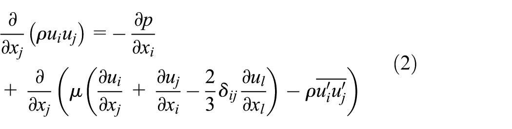
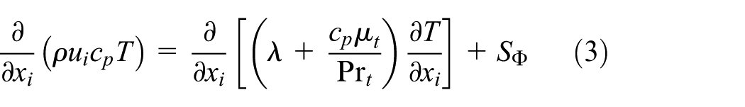
The energy equation is
The species transport equation is

The Boussinesq hypothesis is

The transport equations for the SST k–ω model are as follows

where
A density-based solver with a time-derivative preconditioning was used with an explicit formulation, which solved the governing equations of continuity, momentum, energy, and species transport simultaneously. The convection terms in the governing equations were discretized by the second-order upwind scheme. Roe flux-difference splitting scheme was used for convective fluxes. The convergence criterion for all residuals in the simulation was less than 10−3, with the residual reduced at least three orders of magnitude.
The ideal gas equation of state was used in the simulation. The transport properties such as specific heat, thermal conductivity, and viscosity were calculated using the piecewise-polynomial functions of temperature. The coefficients of the polynomials were defined using the data from the REFPROP of the NIST (National Institute of Standards and Technology). 28
Mass diffusion coefficients were calculated by the kinetic theory using a modification of the Chapman–Enskog formula 29
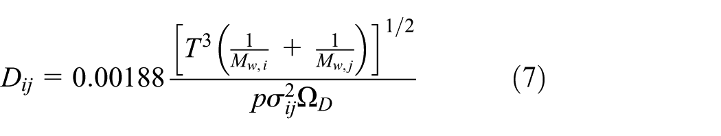
where
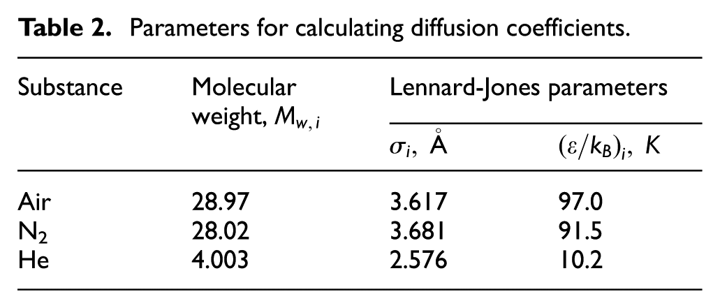
Thermal diffusion coefficients were defined by an empirically based composition-dependent expression derived from ANSYS 29 which caused heavy molecules to diffuse less rapidly, toward heated surfaces
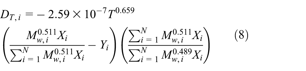
where
Parameters for calculating diffusion coefficients.
Boundary condition and mesh
The specific parameters of the mainstream and film coolant are listed in Table 1. The boundary conditions of the inlet, upper border, and outlet of the mainstream were all set as the pressure-far-field conditions, which can set the subsonic, sonic, or supersonic free stream. The inlet boundary condition of film coolant was set as pressure inlet with a subsonic velocity, which was also set as a laminar condition. The feeding total pressure of the film coolant was set to ensure that the exit pressure of the injection matched that of the free stream, which could have higher effectiveness when compared with the unmatched conditions. 12 The other boundaries were set as walls which were assumed to be adiabatic with no-slip boundary conditions.
A grid-convergence analysis was carried out to test Case 2 in Figure 2. Three grid levels were considered, with 103,489, 481,389, and 615,249 cells, respectively. These grids were refined in the walls and in the step to describe the viscous sublayer, and with the same law of refinement for each grid. The heights of the wall cells for the three grids were set as 0.05 mm (y+ < 3), 0.01 mm (y+ < 0.6), and 0.005 mm (y+ < 0.3), respectively. Figure 2(a) shows the adiabatic temperature of the wall protected by the film coolant under the three grids. The result shows that medium-sized mesh exhibits satisfactory performance in determining the wall temperature.

Results of the three different grid levels: (a) Case 2 and (b) test case of Juhany et al. 15
Using the current grid distribution, three similar grids levels with 63,127, 129,330, and 266,446 cells, respectively, were also used to model the experiments of Juhany et al. 15 The heights of the wall cells were also set as 0.05 mm (y+ < 3), 0.01 mm (y+ < 0.6), and 0.005 mm (y+ < 0.3) for the three grids, respectively. Figure 2(b) shows the comparison of cooling effectiveness between the results obtained using the three grids and the experiments. The modeled cooling effectiveness using the three different grids is constant with the test result. Hence, the medium-sized grid was used in the current numerical simulation.
Validation of the numerical model
Validation with the analytical diffusion problem
Since the supersonic film cooling involved the diffusion of film coolant into the mainstream and the corresponding reverse process, the ability of the current model on demonstrating the diffusion problem should be validated first. A simple diffusion problem of the two gases was used here as shown in Figure 3. The nitrogen and air are isolated by a membrane in an impervious container. When the membrane is removed at time
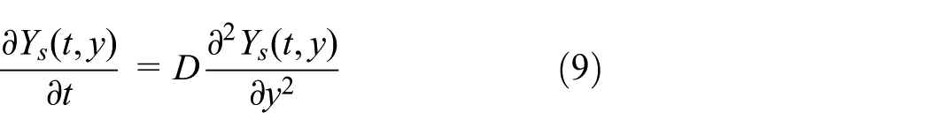
where

The initial condition is
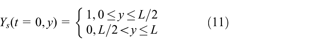
The analytical solution of this problem is as follows


A schematic of diffusion problem.
This diffusion problem was represented with the current model with the actual container sizes of 100 mm in x direction and 200 mm in y direction. Figure 4 shows the comparison of the modeled mass fraction distribution of nitrogen along the y direction between the current model and that of the analytical results. The current model can accurately capture the diffusion of nitrogen into air at different times, so the ability of the model to demonstrate the analytical diffusion problem could be validated. Actually the diffusion condition between the mainstream and film coolant in the supersonic film cooling is convection diffusion, which is greatly different from the analytical problem, so the validation of the analytical diffusion problem can indirectly indicate that the current model can represent the transport of the film coolant for supersonic film cooling.

Comparison of the modeled and analytical solutions of the diffusion problem.
Validation with the experiments
After validating the ability of the model to describe the transport phenomenon, the ability of the numerical method to capture the characteristics of supersonic film cooling should be assessed. Juhany and Hunt 31 measured many pitot pressure profiles of several streamwise locations during their experimental runs. It should be known if the current model could capture these characteristics, so the case 1 of the tests of Juhany and Hunt 31 was modeled with the current numerical method.
Juhany and Hunt 31 presented the boundary layer thickness of the mainstream in their experiments, and the boundary layer state should be modeled first. A precursor simulation was conducted to model the development of the boundary layer of a flat plate. After the precursor simulation, the total pressure profiles of the boundary layer in different streamwise positions were matched with that of Juhany and Hunt, 31 and the specific inflow profile of the current modeling was captured at the best matched streamwise position. The inflow profile at a certain distance before this specific position was then used in the main simulation to make the inflow state of turbulence be matched with that of the experiments.
Figure 5(a) shows the comparison between the modeled pitot pressure profiles at the slot (x/S = 0) in the main simulation with that in the experiment of Juhany and Hunt.
31
The profile near and above the boundary layer is accurately captured, but the profile in the inner boundary layer is not matched well. Figure 5(b) shows the x velocity profile near the wall in the boundary layer, which was rescaled using the van Driest transformation
32
to be compared with the incompressible turbulent boundary layer. The theoretical incompressible law of the wall with

States of inflow at the slot: (a) comparison of numerical pitot pressure profile to the experiment and (b) velocity profile.
Figure 6 presents the comparison of the numerical modeled pitot pressure profiles with those described in the experiment of Juhany and Hunt
31
at different streamwise positions after the step to validate the flowfield after the slot. At x/S = 3, the modeled profile matches the measured profile well at

Comparison of the modeled pitot pressure profiles with the experiment at different streamwise positions.
In film cooling, the temperature of the wall protected by the film coolant is a concern among engineers, so the performance of the model in depicting cooling effectiveness should also be checked. Unfortunately, Juhany and Hunt
31
did not have the available effectiveness data. Experiments from other literature should be used, such as, the test of Juhany et al.,
15
which had the data in need. Figure 7 illustrates the comparison of the modeled film cooling effectiveness with the experiment of Juhany et al.
15
The adiabatic cooling effectiveness was defined as

Comparison of numerical cooling effectiveness with the experiment.
Based on the validation of the current model with the analytical transport problem, experiments of flowfield, and heat transfer in supersonic film cooling, it can be concluded that the current method can be used to model the supersonic film cooling.
Results and discussion
Flow characteristics
The inflow state of the mainstream at the position of the step should be inspected first, as presented in Figure 8(a), which is the profile of Mach number at x/S = 0. The thickness of the boundary layer at this position is 1.7 mm for the Case 1, which is slightly larger than that of 1.1 mm for Cases 2 and 3. As presented above, the film coolant is accelerated by the half Laval nozzle before entering the mainstream. The injecting conditions of the coolant gas, including the distribution of Mach number, total pressure, and total temperature are shown in Figure 8(b)–(d), respectively. The injecting Mach number of the film coolant is mainly distributed near the designed number of 1.5, except for the Case 1, which is a little less than 1.5. The total pressure and temperature of injection of the film coolant are distributed similar to that of the Mach number, and the rapid changes near the upper and lower wall of the slot are due to the development of boundary layers in the respective walls. In general, the current Laval nozzle works to accelerate the film coolant to the designed Mach number.

Profiles of mainstream and film coolant at x/S = 0: (a) Mach number of mainstream, (b) Mach number of film coolant, (c) total pressure of film coolant, and (d) total temperature of film coolant.
Figure 9 shows the static pressure distribution of the three cases near the slot. The overall pressure distributions are nearly the same among the three cases. The static pressure at the outlet of the film nozzle is nearly the same with the mainstream, which shows the film coolant is in matched condition with the mainstream. The flowfield structure in supersonic film cooling after the step is illustrated by the numerical Schlieren image in Figure 10. As shown in Figure 10(a)–(c), the supersonic mainstream flows over the step and expands over the upper tip of the lip, producing a lip expansion fan and a shock wave. There exists also an expansion fan and a shock wave emanating from the lower tip of the lip for the finite thickness of the lip, which are reflected respectively after reaching the wall to be protected. After that, the reflected expansion fan passes through the mixing layer between the mainstream and film coolant and merges with the shock wave emanating from the upper tip of lip in a short distance. The reflected shock wave forms a reattachment shock wave which extends independently downstream. Before the streamwise position of the reattachment of the lower lip shock wave, the laminar boundary layer of film coolant separates and forms a separation bobble near the wall. The mixing layer forms after the lip, and extends almost linearly downstream of the step, despite the interference of the expansion fans and shock waves from the lip. The outlines and positions of the lip shock waves, expansion fans, and reattachment shock wave are almost in the same positions in the three cases, there are no evident differences in the structures of flowfield in these three cases. The flowfield of Cases 1, 2, and 3 in Figure 10 shows an almost similar image.
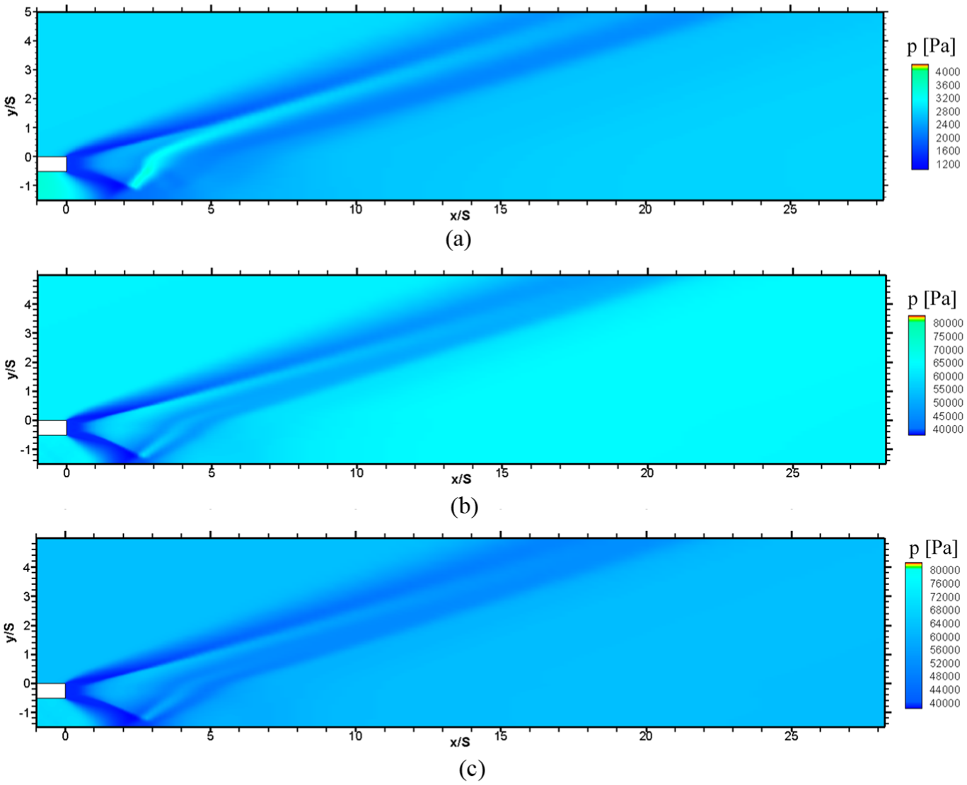
Static pressure distribution near the slot of the three cases: (a) Case 1, (b) Case 2, and (c) Case 3.

Numerical Schlieren image of density gradient in x and y directions: (a) Case 1, (b) Case 2, (c) Case 3, and (d) Case from Konopka et al. 23
The typical schematic flowfield structures of film cooling in the backward-facing step in the vicinity of slot are shown in Figure 11 based on the current numerical results. The typical flowfield structures in Figure 11 are a little different from that of Konopka et al. 23 The numerical conditions same to the work of Konopka et al. 23 were also conducted with the current RANS model to make a comparison, and the modeled flowfield structures near the slot are shown in the numerical Schlieren image in Figure 10(d). As shown in Figure 10(d), the main features of the flowfield structures in the case of Konopka et al. 23 are a little similar with the results of this work except for the different strengths and positions of the upper and lower lip shock waves and expansion fans. The reflected expansion fan emanating from the lower tip of the lip converges to a shock wave in a short distance in their work. A shock forms in the bottom of the film inlet, which may be caused by the fact that the flow of the film coolant in the passage of the slot is not modeled in the simulation. In general, the flowfield structures in the study of Konopka et al. 23 and this work are similar to each other.
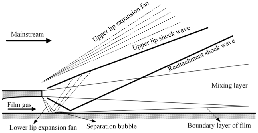
Schematic flowfield structures of supersonic film cooling near the slot.
Heat transfer characteristics
The static temperature field of the supersonic film cooling of the three cases in the current backward-facing step is shown in Figure 12, where the cooled film gas acted as heat barrier between the hot mainstream and the wall to be protected. As the film gas reaches further in the streamwise direction, the overall temperature of the cooling gas increases for it being further mixed with the mainstream. The influence of the lip shock wave and the expansion fan on heat transfer is also visible in the temperature contour in Figure 12.

Contour map of static temperature of (a) Case 1, (b) Case 2, and (c) Case 3.
Figure 13 shows the changes in the adiabatic temperature of the wall to be protected in the three cases, which is also the typical temperature distribution of supersonic film cooling in the backward-facing step. The three curves show small fluctuations before the positions of x/S < 4 because of the interaction of the lip expansion fan and shock wave with the laminar boundary layer of the cooling gas. The wall temperatures remain nearly constant until at certain positions, after which the temperatures begin to increase rapidly.

Adiabatic wall temperature of the plate being protected by the film coolant.
The definition of cooling effectiveness is the same to that reported by Juhany et al. 15 Figure 14 shows the cooling effectiveness calculated using the wall temperatures in Figure 13. The curve remains initially at the value of 1, which extends downstream to a certain distance. The curve then undergoes a transition to an approximate power-law dependence on distance. The turning points in Figure 14 are the same to the adiabatic temperatures of the wall in Figure 13, and this similarity is evident for the definition of effectiveness. These turning points are of considerable concern among engineers for who can easily speculate that the wall before the points can be effectively cooled by the film coolant. In subsonic film cooling, Seban and Back 7 pointed out that the wall temperature remained almost equal to the temperature of the film coolant in the potential region, after that the temperature started approaching that of freestream. Juhany et al. 15 described that the wall jet region started at the position where the mixing layer met the slot flow boundary layer. Considering these representations, we can guess that the turning position corresponds to the border between the potential and wall jet regions, where the mixing layer originating from the lower tip of the lip meets the upper border of the boundary layer of film flow. The characteristics of flowfield at this turning position were not explained by Seban and Back 7 or Juhany et al. 15 in their paper, so this article aims to explain the changes of flowfield at this position and provides detailed information.

Changes in cooling effectiveness and mole fraction of coolant on the wall along streamwise position.
The positions of these turning points in the curves of cooling effectiveness should be defined first. Assume that the curve of effectiveness after the turning point fits a power-law relationship with distance downstream as the Bass et al.,
13
which is also a common practice in experiments of supersonic film cooling. The relationship
Fitting parameters of effectiveness.

Figure 14 shows the changes in the mole fraction of film gas (nitrogen or helium) on the wall protected by the film along the streamwise direction. In the curves of the three cases, the positions where the mole fractions of the film coolant begin to decrease are nearly the same to those of the effectiveness. The calculated mole fractions at the extrapolated turning points are also shown in Table 3. Based on the comparison of the drop rates between the mole fraction and effectiveness at these turning points, the mole fraction in the wall protected by the film drops much faster than that of effectiveness for the Cases 1 and 2 of nitrogen, but nearly has the same speed for the Case 3 of helium.
The flowfield near the extrapolated turning points should be analyzed carefully. Since the turning points in the curves of mole fraction are slightly similar to that of cooling effectiveness, the mole fraction distributions near these turning points are of great concern. Figure 15 shows the contour map of the mole fraction of the mainstream near the turning points of the three cases. The hot mainstream of air reaches the surface of the wall protected by the film coolant at the positions of these turning points, which leads to the decreased cooling effectiveness at these positions. The orders of magnitude of the mole fraction of mainstream near these turning points for the Cases 1 and 2 are 0.1, while it is 0.03 for the Case 3. The streamwise growth rates of mole fraction of the hot mainstream in Cases 1 and 2 at these turning points are much larger than that in Case 3. Because the film coolant of helium have a much larger injecting velocity than that of nitrogen in the same Mach number to make the velocity differences between the mainstream and film coolant be much less, the mixing rate becomes less in Case 3, so less mainstream reaches the wall protected by the film and the effectiveness is dropping much slower in Case 3 than that in Cases 1 and 2 in Figure 14. Based on the work of Peng and Jiang, 33 the improved cooling effect of helium may also be caused by the higher heat capacity of helium than that of air.

Mole fraction contour of air near the turning point in (a) Case 1, (b) Case 2, and (c) Case 3.
Figure 16 shows the streamwise velocity distribution before and after the extrapolated turning points for the three cases. For Case 1, unsmooth transition points are present in each profile where the growth rate of streamwise velocity in y direction changes gradually from an almost constant rate to another before the streamwise position of the extrapolated turning points, such as the points at y/S = −1.35 and y/S = −0.82 for the curve of x/S = 27, y/S = −1.30 and y/S = −0.83 for the curve of x/S = 32. After the extrapolated turning point, only one unsmooth changing point exists where the growth rate of velocity changes gradually, such as the points at y/S = −1.30 for the curve of x/S = 42 and y/S = −1.25 for the curve of x/S = 47. The points near the wall protected by the cooling film, such as the points at y/S = −1.35 for the curve x/S = 27, y/S = −1.30 for the curve of x/S = 32, y/S = −1.30 for the curve of x/S = 42 and y/S = −1.25 for the curve of x/S = 47, are the indicators of the development of boundary layer of the film coolant. These points always exist in the velocity curves before and after the turning points in streamwise direction, which are not of concern in this work, so they are not marked in Figure 16. Whereas the points lying slightly further from the wall, such as y/S = −0.82 for the curve of x/S = 27 and y/S = −0.83 for the curve of x/S = 32 are marked by red pentagrams in the Figure 16, which can be seen as the indicators of the mixed degree between the mainstream and the film coolant. These unsmooth transition points divide the profiles of streamwise velocity into two regions, the region in the wall side protected by the film is only affected by the film coolant, whereas the region in the other side of wall is also affected by the mainstream. The unsmooth transition points in this article are referred to these points. Before the extrapolated turning point in the streamwise direction, the film coolant is not mixed well with the hot mainstream. After the turning point in streamwise direction, these unsmooth transition points disappear from the velocity curve for the mixing between the mainstream and film gas, and the transition of streamwise velocity in the y direction is much smoother. The disappearance of these marked unsmooth transition points in the curves can be seen as the position where the mixing layer meets the slot flow boundary layer. For Case 2 in Figure 16(b), a similar phenomenon exists. The unsmooth transition points away from the wall appears in the profiles of velocity at y/S = −1.05 for the curve of x/S = 17 and y/S = −1.10 for the curve of x/S = 22 before the turning point, which are marked by red pentagram. After the extrapolated turning point, these points disappear. For Case 3 of Figure 16(c), these unsmooth transition points are not sufficient evident, actually the condition here is similar to those in Cases 1 and 2 in the velocity profiles. The points near y/S = 0.82 for the curve of x/S = 53 and y/S = 0.82 for the curve of x/S = 58, which are marked in the figure, disappear in the velocity curves after the turning point in the streamwise direction.

Streamwise velocity distributions near the extrapolated turning points: (a) Case 1, (b) Case 2, and (c) Case 3.
Based on the analysis of the velocity profiles before and after the extrapolated turning point, we can conclude that the extrapolated turning point corresponds to the disappearance of the unsmooth transition points away from the wall where the growth rate of velocity changes from nearly a constant rate to another rate, which also corresponds to the streamwise position where the mixing layer reaches boundary layer of the film coolant.
Given that the unsmooth transition points are present in the profiles of streamwise velocity, other parameters related to the mixing between the mainstream and film coolant are of significant interest. Figures 17 and 18 show the profiles of mole fraction and total temperature distribution before and after the extrapolated turning points, and the trend is similar to that of velocity distribution in Figure 16. For the mole fraction in Figure 17, the unsmooth transition points are located at positions where the growth rate of the mole fraction changes gradually in y direction at y/S = −0.82 for the curve of x/S = 27, y/S = −0.81 for the curve of x/S = 32 for the Case 1 in Figure 17(a), y/S = −1.07 for the curve of x/S = 17, y/S = −1.16 for the curve of x/S = 22 for the Case 2 in Figure 17(b), which are also shown in the figure with red pentagrams. Similar points are not evident for Case 3 in Figure 17(c) than that of velocity in Figure 16(c), so they are not marked in the figure here. The reason is that the drop rate of the mole fraction in the streamwise direction of helium coolant is much slower than that of nitrogen in Cases 1 and 2. Anyway, the transitions in the profiles of the mole fraction after these extrapolated turning points are smooth for the reaching of the mixing region to the wall protected by the film.

Mole fraction distribution of air near the extrapolated turning points: (a) Case 1, (b) Case 2, and (c) Case 3.

Total temperature distributions near the extrapolated turning points: (a) Case 1, (b) Case 2, and (c) Case 3.
The total temperature distribution in Figure 18 shows similar unsmooth transition points, where the growth rate of the total temperature changes at y/S = −0.84 for the curve of x/S = 27, y/S = −0.82 for the curve of x/S = 32 in Case 1, y/S = −1.08 for the curve of x/S = 17, y/S = −1.16 for the curve of x/S = 22 in Case 2, which are all shown as red pentagrams in the figure. The conditions of Case 3 in Figure 18(c) are the same to the profiles in Figure 17(c), where the unsmooth transition points are not evident enough as that of Figure 16(c).
The same unsmooth transition points are found in other parameters, such as density and total pressure, which are not listed here. The small differences between the positions of these unsmooth transition points in different profiles of parameters are due to the interactions among the parameters. Based on the analysis of the flowfield near the turning points, it can be concluded that the extrapolated turning point in the adiabatic wall temperature and also the cooling effectiveness corresponds to the streamwise position where the mainstream reaches the wall protected by the film coolant and also corresponds to the position where the mixing layer meets the slot flow boundary layer. The turning point can also be seen as the border between the potential and wall jet regions. Before the turning point in streamwise direction, the unsmooth transition points are located where the growth rates of the streamwise velocity, mole fraction, total temperature, and other parameters change from a certain condition to another for the cases of nitrogen acting as film coolant. After the turning point in streamwise direction, these unsmooth transition points disappear, and the transitions in the profiles of the parameters become smooth. For the case of light gas of helium, these unsmooth changing points are not sufficiently evident because of the much slower drop rate of effectiveness in the streamwise direction.
Conclusion
Current numerical simulation analyzed the characteristics of flowfield and the heat transfer in supersonic film cooling ejected through a half Laval nozzle set in a backward-facing step. Three cases are considered to represent three typical conditions. This work aims to explain the typical mechanics of heat transfer in the current configuration of supersonic film cooling, especially the flowfield changes near the turning point in the wall temperature or the cooling effectiveness curve. The turning point is defined by the extrapolation of the cooling effectiveness curve using a power-law relationship. The extrapolated turning point corresponds to the disappearance of the unsmooth transition points away from the wall where the growth rate of streamwise velocity changes from a certain condition to another, and to the streamwise position where the mainstream reaches the wall protected by the film, and the position where the mixing layer meets the boundary layer of the film coolant. Before the extrapolated turning point, the unsmooth transition points are present in the curves of streamwise velocity, mole fraction, and total temperature and also other parameters where the growth rates change from a certain condition to another for cases of nitrogen. These points are not evident for the case of a light coolant of helium due to the slow drop rate of effectiveness.
Footnotes
Appendix 1
Acknowledgements
The authors thank the anonymous reviewers for some very critical and constructive recommendations on this article.
Handling Editor: Ruey-Jen Yang
Declaration of conflicting interests
The author(s) declared no potential conflicts of interest with respect to the research, authorship, and/or publication of this article.
Funding
The author(s) disclosed receipt of the following financial support for the research, authorship, and/or publication of this article: The authors would like to express their thanks for the support from the National Natural Science Foundation of China (Grant No. 11572346).