Sage Journals: Discover world-class research

Abstract

The mathematical model of the initial pipeline and cable process is created with regard to the ocean current load and wave load; and the mathematical model is solved by the numerical quasi-Newton method to investigate the effects of the current and wave load on the shape and force of the pipeline and cable during the initial pipe-laying process. On this basis, semi-physical simulation system is built to visualize the initial pipe-laying process. The simulation results are compared with OFFPIPE’s results to verify the mathematical model. The current and wave load effects on the shape and tension of the pipeline and cable are analyzed. This real-time virtual reality system will help engineering project in risk management and prediction as well as staff training, which is of vital significance for minimizing the risk of the actual pipe laying and improving the efficiency of the pipe-laying work.

Keywords

Initial pipe laying quasi-Newton method numerical solution interactive simulation virtual reality

Introduction

To exploit offshore oil and gas, the offshore gas pipeline has been employed. In 1954, Brown and Root laid the world’s first submarine pipeline in the Gulf of Mexico in the United States. So far, there are about 3800 oil and gas pipelines in active service around the world. The marine environment is complicated and inconstant; thus, the operation environment is a big challenge for pipe laying, and any incorrect manipulation tends to produce irreparable damage as well as the project postponed. The initial pipe laying of submarine pipelines¹ is the process of laying down the pipe to the designated area of the seabed under initial cable traction. During this process, it is necessary to predict the state of the pipe and cable simultaneously. Currently, most studies ware focused on the analysis of the shape and force of S-lay pipes and stand pipes during the normal laying^2,3 process, whereas few studies reported on the cable- and pipe-coupled system during the initial laying process under ocean current load. W He et al.⁴ analyzed seabed stand pipes and conducted a detailed study on the calculation method of the differential equation of pipelines, while L Zhi-Gang et al.⁵ adopted the difference method to solve the pipeline mechanics model. Furthermore, Z Kang et al.⁶ simplified and modified the calculation based on the traditional natural catenary algorithm. According to different situations and boundary conditions, Ma Xiaoyan⁷ proposed the segmental treatment of the S-lay pipeline shape and used different algorithms to calculate the upper bend section, middle section, and lower bend section of the pipeline.

Virtual reality (VR) technology is computer simulation systems to virtually create and allow people to experience something or environment in the virtual world. From the 1950s to late 1970s, it was the exploration stage of VR technology. From the early 1980s to the mid-1980s, VR technology became more systematic and moved forward from the laboratory to application. From the late 1980s to the early 21st century, VR technology experienced a quick development.⁸ VR technology has been widely used in the United States and other Western countries,^9,10 in particular, Norway and Canada have applied pipe-laying visual simulation technology in engineering projects.¹¹ VR for the pipe laying of submarine pipelines has been studied by Harbin Engineering University and North western Polytechnical University^12,13 in China.

The research objective is to develop a VR-based pipe-laying simulation system that will strongly support engineering projects in the following areas: first, the initial pipe-laying simulation system will enable the full rehearsal of the actual pipe-laying operation cases, identify the possible issues in time, and approve the actual pipe-laying operation plan; second, the pipe-laying simulation system will output the real-time pipeline shape and stress parameters as well as the motion of the pipe-laying ship, help to accurately set and input the key parameters during the process of the pipe-laying operations, and thus provide the reliable reference for decision-making in the actual operation plans; in the end, the initial pipe-laying simulation system can be used in the technical personnel training for pipe laying.

The big challenge of this research is that the VR system must have a good accuracy and a real-time response or in other word, the computation time must be negligible compared with system response time, which is on a second level. Finite element method (FEM)-based simulations can predict strain/stress very well, but the computation tends to introduce a unacceptable delay and cannot compute the ship motion. Multiple-body-based simulation will introduce a big item delay as well, and the post-process will cost a long time, which makes it only suitable for well-trained professionals. Meanwhile, the operation panels must agree with the real system, which could not be virtualized.

This study is based on the real pipe-laying operation of the deep-water pipe-laying vessel named “Offshore Oil 201.” On the basis of the Euler–Bernoulli beam theory,^14,15 the initial pipe-laying mathematical model of the pipeline is established. In addition, according to the characteristics of differential equations, the quasi-Newton method^16,17 is used to solve the equations in real time. The dynamic response of the pipeline and cable system is obtained under the current load and wave load. According to the data and process of the real pipe-laying operation of the deep-water pipe-laying vessel, representative pipe-laying cases are simulated. The simulation results are compared to those of the commercial software OFFPIPE,¹⁸ and the errors are less than 5%.

Interactive simulation system for deep-water pipe laying

Pipe-laying operation system

The schematic diagram of the pipe-laying system is shown in Figure 1. This system consists of a dynamic positioning system (DP system) and a pipe-laying system. While the DP system will control the ship’s movement and positioning, the pipe-laying system includes a production line for onboard pipe prefabrication, a tensioner system, and a stinger. The production line connects single 12-m-long steel pipes into a continuous pipeline by cutting, beveling, and welding. The tensioner system consists of a tensioner and a winch, in which the tensioner will pull the pipe and utilizes the track to lower down or withdraw the pipeline. The winch will lower or withdraw the cable. As an important supporting device for the S-lay pipe laying, the stinger controls the curvature of the pipeline during the process and prevents the pipeline from buckling due to excessive bending moment to ensure the safely laying of the pipeline.

Figure 1.

Pipe-laying ship.

The initial pipe-laying process is shown in Figure 2. One end of the cable is fixed on the designated seabed by an anchor, and the other end is connected with the end of the pipe. The tension and speed of the pipe laying are controlled by the tensioner. The pipe-laying ship keeps moving by the cooperation of the DP system and tensioner, and continuously lays down the pipe to the seabed under the traction of the cable until the initial pipe-laying operation finishes.

Figure 2.

Initial pipe-laying process.

Pipe-laying simulation system

The pipe-laying simulation system consists of seven parts: tensioner remote console, master server, visual server, DP console, a network switch, coach console, and stereoscopic projection device. The simulation system structure is shown in Figure 3. The coach system, visual server, and master server are connected into an internal sub-network by the switch.

Figure 3.

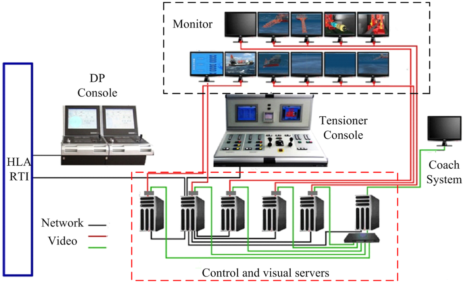
Pipe-laying simulation system.

The laying and withdrawing of the pipeline and cable can been achieved through the tension control system of tensioner remote console. The force and speed double closed-loop control is used according to the difference between the preset tension and the actual tension, as well as the difference of the ship speed and the pipe-laying rate, to ensure the safety of the pipe laying and withdrawing.

The master server is the core of the pipe-laying simulation system. The mathematical model of the pipe-laying operation is embedded in the master server in the form of C++. It is responsible for all the data communication and calculation related to pipelines and cables in the pipe-laying operation. The visual server is responsible for the communication and calculation of the visual data. The display can be updated in real time according to the data from the DP console, the tensioner remote console, and the master server. Dual-channel three-dimensional (3D) projection is used in the stereo projection equipment to present the virtual environment of pipe-laying ship in front of the operator.

DP console is the ship motion control system. It is responsible for the marine environmental parameters calculation and hull movement control. DP console will calculate the ship’s position and attitude, and drive the hull in accordance with the control instructions in manual mode, automatic positioning mode, or tracking mode.

The coach console is the top control unit of the pipe-laying simulation system with the highest priority. The coach console will set up initial parameters and simulation cases, and monitor all of the data and visual screens of the pipe-laying simulation system in real time. The switch is a data transfer station for the network communication. The coach console can invoke all of the data obtained in the process of pipe-laying through the switch. The network structure is shown in Figure 4.

Figure 4.

Network of pipe-laying simulation system.

Establishment of virtual environment

The virtual environment system is used to simulate the pipe-laying ship and its operating environment. Through the multi-channel technique, the visual image is projected on the screen and the realistic image is presented to the trainees, allowing trainees to perceive the pipe-laying environment. This system consists of two parts: one part is the drive module and the other part is the unified 3D model database established according to the unified standards and regulations. The relationship between the drive module and the 3D model database is shown in Figure 5. The left part is the construction process of 3D model database of the virtual environment system. The right part is the composition of the drive module, which processes the 3D model in the database and produces the 3D visual effect through a stereographic projection device. All 3D models of the virtual environment are built and rendered by 3DMax,¹⁹ and the drive is developed on the basis of the Quest 3D platform.²⁰

Figure 5.

Schematic diagram of the visual display system for pipe-laying operation.

Mathematical model of initial pipe laying

The modeling of the initial pipe-laying operation is composed of pipe-laying system modeling and ship motion system modeling.

Ship motion system modeling

The ship coordinate system is shown in Figure 6. The origin of the world coordinate system O_nX_nY_nZ_n is a fixed point, and OXYZ is the ship coordinate system.

Figure 6.

Ship coordinate system.

Force equation of the crane ship is²¹

M_{RB} \overset{\cdot}{v} + C_{RB} (v) v = τ_{RB}

(1)

where M_RB is the mass matrix, v = [u, κ, w, p, q, r]^T is the general velocity and general angular velocity, τ_RB = [X, Y, Z, K, M, N] is the general force and general moment, and C_RB is the Coriolis–centripetal force matrix.

Hydrodynamics is necessary to be involved in the hull modeling.²² When the hydrodynamic added mass and hydrodynamic damping are involved in, the model of the ship can be rewritten as

\begin{matrix} M_{RB} \overset{\cdot}{v} + C_{RB} (v) v + M_{A} {\overset{\cdot}{v}}_{r} + C_{A} (v_{r}) v_{r} + D (v_{r}) v_{r} \\ = τ_{wind} + τ_{wave} + τ_{current} + τ_{control} \end{matrix}

(2)

where $M_{A} {\overset{\cdot}{v}}_{r} + C_{A} (v_{r}) v_{r}$ is the hydrodynamic force, M_A is the hydrodynamic added mass matrix, C_A is the Coriolis–centripetal force matrix caused by the hydrodynamic added mass, D(v_r)v_r is the hydrodynamic damping force, D(v_r) is the hydrodynamic damping matrix, v_r is the relative velocity between hull and seawater. g_B is the force produced by the ballast system, τ_wind is the wind load, τ_wave is the wave load, τ_current is the current load, and τ_control is the general control force.

Mass matrix of the ship, including the hydrodynamic added mass, is

M_{RB} = [\begin{matrix} M & 0 & 0 & 0 & M . Z_{GC} & - M . Y_{GC} \\ 0 & M & 0 & - M . Z_{GC} & 0 & - M . X_{GC} \\ 0 & 0 & M & M . Y_{GC} & - M . X_{GC} & 0 \\ 0 & - M . Z_{GC} & M . Y_{GC} & I_{44} & I_{45} & I_{46} \\ M . Z_{GC} & 0 & - M . X_{GC} & I_{54} & I_{55} & I_{56} \\ - M . Y_{GC} & M . X_{GC} & 0 & I_{64} & I_{65} & I_{66} \end{matrix}]

(3)

where M is the sum of the ship mass and added mass; I_ij(i = j) is the inertia moments about the O_bx axis, O_by axis, and O_bz axis; and I_ij(i ≠ j) is the inertia products on the O_bxy plane, O_byz plane, and O_bzx plane.

The mass matrix M_RB can be expressed in the following

M_{RB} = M_{RB}^{T} = [\begin{matrix} M_{11} & M_{12} \\ M_{22} & M_{22} \end{matrix}] > 0

(4)

Thus, the Coriolis–centripetal force matrix is

C_{RB} (v) = [\begin{matrix} 0_{3 \times 3} & - M_{11} v_{1} + M_{12} v_{2} \\ - M_{11} v_{1} + M_{12} v_{2} & - M_{21} v_{1} + M_{22} v_{2} \end{matrix}]

(5)

where v₁ = [u, κ, w]^T is the line velocity vector and v₂ = [p, q, r]^T is the angular velocity vector.

Mathematical model of the environmental load

Current load

In the calculation of the deep-water pipe laying, the current load is generally regarded as a constant current, of which the flow direction remains unchanged in a period of time. The following formula is used to calculate the current velocity below the sea surface²³

v = v_{m} \frac{h}{H} + v_{t} {(\frac{h}{H})}^{\frac{1}{7}}

(6)

where v_m is the wind velocity of the sea surface (m/s), v_t is the velocity of the tidal flow on sea surface (m/s), H is the depth of the water (m), and h is the depth of the ocean current to the seabed (m).

Based on the current data of the South China Sea, the force of the current acting on the pipeline can be idealized as a steady gradient force, which gradually decreases from the top to the sea bottom. This gradient current force is a drag to the pipeline caused by the flow of seawater

F_{c} = \frac{1}{2} D ρ C_{D} v^{2}

(7)

where F_c is the current load on the unit tube (N), v is the maximum current velocity (m/s), ρ is the density of the seawater (kg/m³), D is the outer diameter of the pipeline (m), and C_D is the drag coefficient of the pipeline.

The drag force on the tube of unit length caused by the current is

F_{d} = \frac{π ρ C_{M} D^{2}}{4} \frac{d v}{d t}

(8)

where C_M is the inertial force coefficient of the pipeline.

The force produced by the current is shown in Figure 7.

Figure 7.

Current drag force on unit tube length.

By equations (6) and (8), the current load of the pipeline can be expressed as

{\begin{matrix} F_{xn} = \frac{1}{2} D ρ C_{D} v \cos β \sin θ ‖ v \cos β \sin θ ‖ \\ F_{xt} = \frac{1}{2} D ρ C_{D} v \cos β \cos θ ‖ v \cos β \cos θ ‖ \\ F_{y} = \frac{1}{2} D ρ C_{D} v \sin β ‖ v \sin β ‖ \end{matrix}

(9)

where β is the current direction, and θ is the inclination angle of the tube unit.

Wave load

In the process of pipe laying, it is difficult to establish an accurate mathematical model of the wave load due to the influence of complex ocean environment. At present, the analysis of irregular waves is usually classified as the designed wave method and probability distribution method. Because of the complexity of irregular waves, the designed wave method is usually used to express the waves in marine engineering. The popular theories include linear wave theory, nonlinear wave theory, and the small amplitude wave theory.²⁴ Since S-lay pipe laying is operated in deep water, the seabed depth is approximately uniform, and the wave height is much less than the seabed depth. Hence, the linear wave theory can be used to model the wave load.

According to the linear wave theory, the horizontal and vertical water particle velocity in the wave field can be expressed as²⁵

{\begin{matrix} u_{x} = ω A e^{kz} \cos (kx - ω t) \\ u_{z} = ω A e^{kz} \sin (kx - ω t) \end{matrix}

(10)

where A is the amplitude of the wave surface; k is the wave number (k = 2π/λ); λ is the wave length; ω is the wave frequency, ω = 2π/T_a, T_a is the period of wave, $T_{a} = \sqrt{2 π λ / g} \approx 0.8 \sqrt{λ}$ .

Differentiate equation (10) with respect to t

{\begin{matrix} a_{x} = kAg e^{kz} \sin (kx - ω t) \\ a_{z} = - kAg e^{kz} \cos (kx - ω t) \end{matrix}

(11)

In submarine pipeline laying, D/λ << 0.2. Therefore, the Morrison equation²⁶ can be used to calculate the wave load. The inclined pipeline stress under wave load is shown in Figure 8, where ζ is the pipe inclination angle, and the wave direction angle is ξ to the x-axis.

Figure 8.

Inclined pipeline stress under wave load.

As shown in Figure 8, the wave velocity on the pipeline can be decomposed into U_n and U_t, and the acceleration can be decomposed into a_n and a_t. Since they are not in the same plane, the wave force needs to be calculated by the vector in the drag force and inertial force. The Morrison equation is generally expressed as

f = \frac{1}{2} C_{D} ρ D U_{n} | U_{n} | + C_{M} ρ \frac{π D^{2}}{4} a_{n}

(12)

In equation (12), f is the wave force vector of the tube of unit length (N), U_n is the normal wave velocity vector (m/s), a_n is the normal wave acceleration vector (m/s²), |U_n| is the modulus of the velocity vector, U_n, C_D is the drag force coefficient, and C_M is the inertial force coefficient.

Pipeline mathematical model

Static force analysis of the pipeline

A micro pipeline segment is analyzed, and the equilibrium differential equation of the micro pipeline segment is established under the natural coordinate system (θ, s),²⁷ as shown in Figure 9.

Figure 9.

Stress analysis of micro pipeline segment.

The equilibrium differential equation is

f (s) = f_{0} \sin θ = \frac{1}{2} D ρ C_{D} v | v | \sin θ

(13)

According to force balance at the point of connection between the pipe and the cable

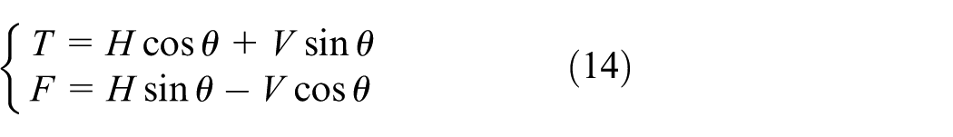
{\begin{matrix} T = H \cos θ + V \sin θ \\ F = H \sin θ - V \cos θ \end{matrix}

(14)

where F is the pipe shear force component, T is the pipe tension, H is the horizontal tension at the connection point of pipeline and cable, V is the vertical force at the connection point, and θ is the tube unit inclination angle.

The normal force along the central line can be decomposed as

dF - Td θ + w \cos θ ds + f (s) ds = 0

(15)

where f(s) is the external current load and w is the pipe weight in seawater per meter.

According to coordinate incremental geometric relationship of the micro pipeline segment

ds = \frac{dx}{\cos θ} = \frac{dy}{\sin θ}

(16)

Derive formula (15) for s

\frac{dF}{ds} - T \frac{d θ}{ds} + w \cos θ + f (s) = 0

(17)

In pipe laying, the length of pipeline is much more than the section dimension (diameter) of the pipeline, which can be treated as a beam. The available analytical theories of beam analysis include Euler–Bernoulli theory and Timoshenko theory.²⁸ Two hypotheses are employed in the Euler–Bernoulli beam theory for the analysis of the beam deformation: (1) the section plane vertical to the centerline will keep flat after deformation (rigid cross section assumption) and (2) the section plane will keep vertical to the deformed axis after deformation. The Timoshenko beam theory takes into account the rotation and shear deformation of the cross section of the beam, which is suitable for beam slab bridges of shorter effective length or of composite materials. The pipeline is a beam with large slenderness ratio (>100 beams), and the shear deformation and rotation of cross section can be neglected, which will save computation time to make the system more close to real time. By the beam theory²⁹

M = EI \frac{d θ}{ds}, F = \frac{dM}{ds}

(18)

where EI is bending rigidity of the pipeline, and M is bending moment of the pipeline.

Substitute equation (18) into (17) yields

EI \frac{d^{3} θ}{d s^{3}} - T \frac{d θ}{ds} + w \cos θ + f (s) = 0

(19)

Vibration of the pipeline

The vibration of the pipeline in the vertical plane is as shown in Figure 10, where V is pipe-laying velocity, the origin is the outlet of stinger, x is the pipe central line, y is the normal direction and literal vibration is neglected, P is axial force, and l(t) is pipe length.

Figure 10.

Pipeline vibration analysis.

Suppose the pipe-laying velocity is constant and

\frac{\partial x}{\partial t} = V, \frac{dV}{dt} = 0

(20)

The vibration velocity of the pipeline can be expressed as

\frac{dy (x, t)}{dt} = \frac{\partial y}{\partial x} \frac{\partial x}{\partial t} + \frac{\partial y}{\partial t} = V \frac{\partial y}{\partial x} + \frac{\partial y}{\partial t}

(21)

The total kinetic energy of the pipeline is

W = \frac{1}{2} ρ Al V^{2} + \frac{1}{2} ρ A \int_{0}^{l} {(V \frac{\partial y}{\partial x} + \frac{\partial y}{\partial t})}^{2} dx

(22)

where A is the cross-sectional area, and ρ is the density.

The total potential energy of the pipeline is

U = \int_{0}^{l} [\frac{1}{2} P {(\frac{\partial y}{\partial x})}^{2} + + \frac{1}{2} EI {(\frac{\partial^{2} y}{\partial x^{2}})}^{2}] dx

(23)

where E is Young’s modulus, and I is the cross-sectional moment of inertia.

In variation, equation (22) can be rewritten as

δ W = ρ AV \int_{0}^{l} (V y_{x} + y_{t}) δ y_{x} dx + ρ A \int_{0}^{l} (V y_{x} + y_{t}) δ y_{t} dx

(24)

According to the Hamilton principle,³⁰ the pipeline vibration differential equation³¹ can be obtained after the higher order terms neglected

EI \frac{\partial^{4} y}{\partial x^{4}} + ρ A \frac{\partial^{2} y}{\partial t^{2}} + 2 ρ AV \frac{\partial^{2} y}{\partial x \partial t} + ρ A V^{2} \frac{\partial^{2} y}{\partial x^{2}} - P \frac{\partial^{2} y}{\partial x^{2}} = 0

(25)

where $EI (\partial^{4} y / \partial x^{4})$ represents the section shear caused by bending, $ρ A (\partial^{2} y / \partial t^{2})$ is the lateral acceleration inertial force, $2 ρ AV (\partial^{2} y / \partial x \partial t)$ is the Coriolis acceleration inertia force, $ρ A V^{2} (\partial^{2} y / \partial x^{2})$ is the centripetal acceleration inertia force, and $P (\partial^{2} y / \partial x^{2})$ represents the component in y of the axial resultant.

If the pipeline damping force and the external load are taken into account, equation (25) is expressed as

\begin{array}{l} E I \frac{\partial^{4} y}{\partial x^{4}} + ρ A \frac{\partial^{2} y}{\partial t^{2}} + 2 ρ A V \frac{\partial^{2} y}{\partial x \partial t} + ρ A V^{2} \frac{\partial^{2} y}{\partial x^{2}} \\ - P \frac{\partial^{2} y}{\partial x^{2}} + c \frac{\partial y}{\partial t} = q (x, t) \end{array}

(26)

where c is the damping coefficient, q(x, t) is the wave load, which includes drag force and inertial force.

The equivalent damping coefficient can be deduced on the base of the motion of the ship in the wave, and the motion of the regular wave is used to take place on the motion of the ship. The equivalent damping coefficient can be expressed as³²

c = \frac{2 k ρ_{w} D C_{D} ω^{2} H e^{nz}}{3 π}

(27)

where k is the control parameter, ω is the wave circular frequency (rad/s), H is the weight height (m), n is the wave number, z is the depth of the water (m), D is the outer diameter of the pipeline (m), and ρ_w is the density of the seawater (kg/m³).

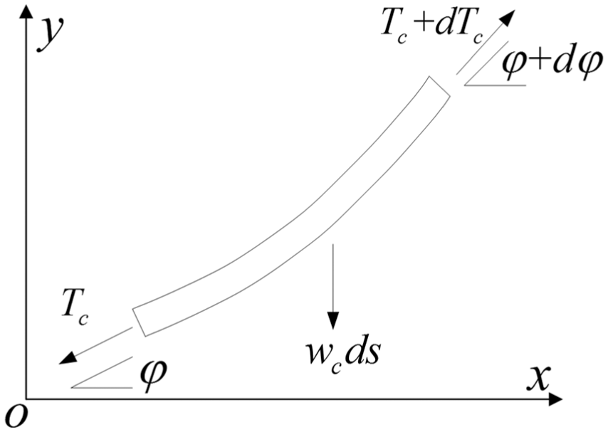
Stress analysis of the cable

The cable is also subjected to stress analysis using micro segments. The length of the micro segment is ds, and the tension at both ends is T_c and T_c + dT_c, respectively. The weight of the cable will increase the axial tension of the pipe, and an angle increment dφ is introduced (Figure 11).

Figure 11.

Stress analysis of the micro cable segment.

Neglecting the influence of the current load on the cable,³³ the axial force equilibrium equation of the cable is

(T_{c} + d T_{c}) = w_{c} ds \sin φ + T_{c}

(28)

where w_c is the weight of unit length of cable in seawater, and φ is the unit inclination angle of the cable.

The weight w_c of a cable can be calculated as

w_{c} = \frac{π {D_{c}}^{2}}{4} g (0.7 ρ_{c} - ρ_{w})

(29)

where D_c is the cable diameter (m), ρ_c is the steel density of the cable (kg/m³), and ρ_w is the density of the seawater (kg/m³).

Divide the initial cable into n segments from top to bottom, the length of each segment is S_i, and the axial forces at both ends are T_ci and T_ci+₁. Then, the axial force relation between point i and point i + 1 is

T_{ci + 1} = \sqrt{{T_{ci}}^{2} - {(w_{c} s_{i} \cos φ_{i})}^{2}} - w_{c} s_{i} \sin φ_{i}

(30)

The inclination angle relation between point i and point i + 1 is

φ_{i + 1} = φ_{i} - d φ_{i} = φ_{i} - \frac{w_{c} s_{i} \cos φ_{i}}{T_{c}}

(31)

The incremental relation in the pipe micro segment coordinate is

{\begin{matrix} d x_{i} = s_{i} \cos φ_{i} \\ d y_{i} = s_{i} \sin φ_{i} \end{matrix}

(32)

Numerical algorithm

Discrete differential equation

Define the following non-dimensional coefficients

z = \frac{s}{L}, x = \frac{X}{L}, t = \frac{T L^{2}}{EI}

(33)

where L is the length of the pipeline, I is the moment of inertia, and E is Young’s modulus.

Equation (15) and (19) can be rewritten as

t_{i} = - \frac{L^{3} h}{EI} \sum_{0}^{i - 1} (w \sin θ_{j} - f_{0} \cos θ_{j}) + t_{0}

(34)

t_{i} = - \frac{L^{3} h}{EI} \sum_{0}^{i - 1} (w \sin θ_{j} - f_{0} \cos θ_{j}) + t_{0}

(35)

The difference scheme of differential equation (34) is

t_{i} = - \frac{L^{3} h}{EI} \sum_{0}^{i - 1} (w \sin θ_{j} - f_{0} \cos θ_{j}) + t_{0}

(36)

Equation (36) can be iterated to obtain the internal force of the pipe node

t_{i} = - \frac{L^{3} h}{EI} \sum_{0}^{i - 1} (w \sin θ_{j} - f_{0} \cos θ_{j}) + t_{0}

(37)

Equation (35) can be discretized as

\begin{array}{l} \frac{E I}{2 h^{3} L^{3}} θ_{i + 2} - (\frac{E I}{h^{3} L^{3}} + \frac{E I t}{2 L^{3} h}) θ_{i + 1} + w \cos θ_{i} \\ + (\frac{E I}{h^{3} L^{3}} + \frac{E I t}{2 L^{3} h}) θ_{i - 1} - \frac{E I}{2 h^{3} L^{3}} θ_{i - 2} + f (s_{i}) = 0 \end{array}

(38)

Numerical solution of equations

The nonlinear equations cannot be solved by analytical method, and the numerical solution of the equation set can be obtained by iteration. Available numerical iterative methods include direct iteration method, Newton method, secant method, and quasi-Newton method. The convergence of the direct iteration method is very slow. The Newton method and secant method are more efficient, but the monotonicity of the criteria needs to be judged, and the iteration may not converge at some boundary points. The quasi-Newton method does not require derivation and the monotonicity of the criterion. The calculation is quick enough to be used in real-time simulation.

After the differential equation is discretized, the numerical method can be used to define the difference of the pipeline and obtain the differential equilibrium equation

\begin{matrix} G (θ_{i}) = \frac{EI}{2 h^{3} L^{3}} θ_{i + 2} - (\frac{EI}{h^{3} L^{3}} + \frac{EIt}{2 L^{3} h}) θ_{i + 1} + w \cos θ_{i} \\ + (\frac{EI}{h^{3} L^{3}} + \frac{EIt}{2 L^{3} h}) θ_{i - 1} - \frac{EI}{2 h^{3} L^{3}} θ_{i - 2} + f (s_{i}) = 0 \end{matrix}

(39)

The above equation can be rewritten as

θ = {(θ_{1}, θ_{2}, \dots, θ_{n})}^{T}

(40)

Define the vectors $θ = (θ_{1}, θ_{2}, \dots, θ_{n})^{T}$ and $F = (G_{1}, G_{2}, \dots, G_{n})^{T}$ , the above formula can be written as

s^{k} = θ^{k + 1} - θ^{k}

(41)

Define $s^{k} = θ^{k + 1} - θ^{k}$ and $y^{k} = F (θ^{k + 1}) - F (θ^{k})$ , the Inverse Broyden equation is

{\begin{matrix} θ^{(k + 1)} = θ^{(k)} - H_{k} F (θ^{(k)}) \\ H_{k + 1} = H_{k} + (s_{k} - H_{k} y_{k}) \frac{{(s_{k} - H_{k} y_{k})}^{T}}{{(s_{k} - H_{k} y_{k})}^{T} y_{k}} \end{matrix}

(42)

The algorithm of equation (42) is

Step 1. Initialize $θ_{0} \in R^{n}$ and the step coefficients of $ε_{1}$ and $ε_{2}$ ;

Step 2. Calculate initial matrix $H_{0} \in R^{nn}$ , $H_{0} = [F' (θ_{0})]^{- 1}$ , or unit matrix $I$ ;

Step 3. $k = 0$ , calculate $F (θ_{0})$ ;

Step 4. Calculate $s_{k} = - H_{k} F (θ_{k})$ , $θ^{k + 1} = θ^{k} + s^{k}$ ;

Step 5. Calculate $F (θ^{k + 1})$ , if the result is $| | F (θ^{k + 1}) | | < ε_{1}$ or $| | s_{k} | | \leq ε_{2}$ , turn to Step 8, otherwise, carry on Step 6;

Step 6. Calculate $y^{k} = F (θ^{k + 1}) - F (θ^{k})$ and get $H_{k + 1}$ by calculating equation (40);

Step 7. $k = k + 1$ , turn to Step 4;

Step 8. $θ^{*} = θ^{k + 1}$ , the iteration is finished.

From the above analysis, the tension $(H_{0})$ provided by the tensioner is required to iterate the shape of the pipeline. When the maximum bending moment $(M_{\max})$ of the pipe section is set, the tension value $(H_{0})$ of the tensioner at every stage of the initial pipe-laying operation is determined to ensure that the buckling of the pipe will not occur. A tension value $(H_{m})$ is initially calculated as the preset value of the tensioner. By substituting the preset value into the differential equation, the corresponding shape and maximum bending moment $(M_{0})$ of the pipe can be obtained. The maximum bending moment $(M_{0})$ obtained by iteration is compared with the ultimate bending moment $(M_{\max})$ , if the ratio is small, the preset value $(H_{m})$ of the tensioner is therefore the required tension value; otherwise, the $H_{m}$ value needs to be adjusted correspondingly according to $M_{0}$ , if $M_{0} > M_{\max}$ , the preset tension value should be increased; otherwise, the preset tension value is reduced. The differential equations are solved with this tension value, and the shape and internal force of the pipeline and cable are calculated as well. The calculation process is shown in Figure 12.

Figure 12.

Initial pipe-laying iterative calculation flowchart.

Simulation cases and analysis

Initial pipe-laying process

The simulation example is based on the actual submarine pipeline laying process. The specific initial pipe-laying simulation process is as follows:

Step 1: The anchor and the cables are placed to the seabed, and the starting position of the pipe-laying is determined (Figure 13);

Step 2: Install the initial head and connect the pipe and the cables (Figure 14);

Step 3: Pipes are prefabricated onboard (Figure 15);

Step 4: The pipe is released by the tensioner in constant tension mode, and the ship’s movement is controlled by DP system (Figure 16).

Step 5: Keep piping until the pipe contacts the seabed, thus, the pipeline laying process changes to the normal pipe-laying mode (Figure 17).

Figure 13.

The initial anchor and cable: (a) initial anchor installation and (b) initial cable.

Figure 14.

Connection of pipe and initial cable: (a) initial head and (b) connection of pipe and initial cable.

Figure 15.

Pipe prefabrication: (a) pipeline alignment, (b) foundation welding, (c) fill welding, (d) AUT flaw detection, (e) sandblasting, and (f) seal coating.

Figure 16.

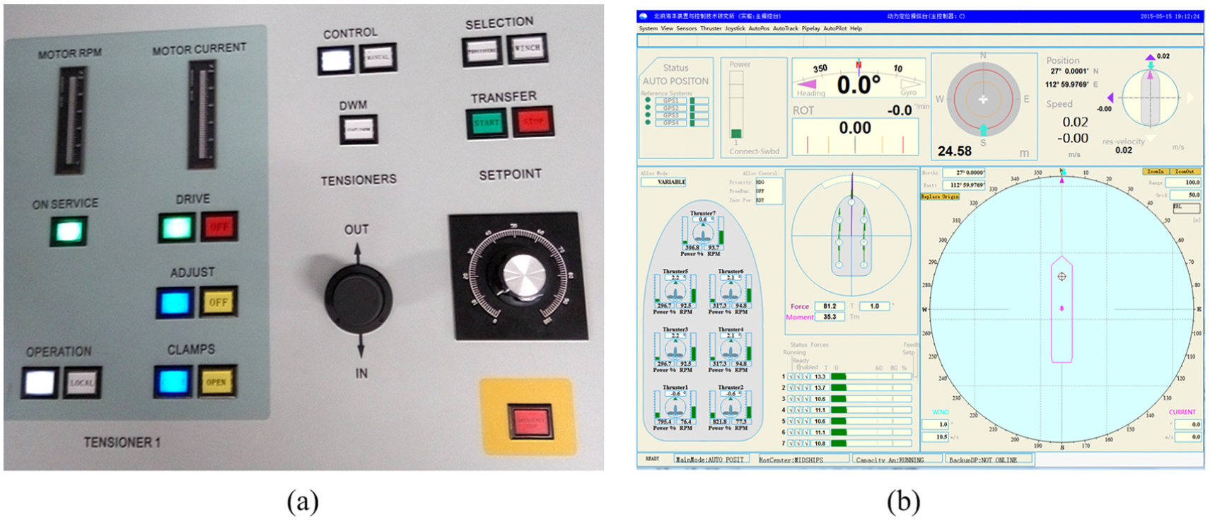
Tensioner system and DP system: (a) tensioner constant tension mode and (b) DP system control interface.

Figure 17.

The pipeline: (a) the pipeline on the stinger and (b) the side view of laying pipe.

Comparison and verification

In order to verify the accuracy of the pipe-laying simulation system, the simulation results are compared with those of OFFPIPE in the same environment with the same pipe and cable parameters. OFFPIPE is the most authoritative software in the offshore oil industry,³⁴ despite its high computational precision; its calculations are too slow to be used in a VR.

The environment parameters and pipeline and cable parameters of the simulation case are listed in Tables 1 and 2:

Table 1.

Piping simulation case initial environmental parameters.

Pipeline parameters	Value
Maximum depth of water	1000 m
Wind velocity	2.5 m/s
Wave height	2 m
Current velocity	0.31 m/s
Flow direction	22.5°
Spectral peak period	8 s

Table 2.

Pipeline and cable parameters.

Pipeline and cable parameters	Value
Pipe OD	168.27 mm
Pipe wall thickness	12.7 mm
Floating weight	25.7 kg/m
Yield strength	430.1 MPa
Single pipe length	12.2 m
Pipeline material density	7850 kg/m³
Elastic modulus of the steel pipe	2E11 Pa
Cable density	7850 kg/m³
Cable OD	35 mm
Cable elastic modulus	2.03E11 Pa
Radius of the curvature of the stinger	75 m

OD: outside diameter.

Figure 18 shows the shapes of the pipeline and cables when the pipeline length L is 200, 400, 600, and 1000 m. The data collected from the simulation are compared with OFFPIPE. The results are plotted in Figure 18(a)–(d).

Figure 18.

Pipeline and cable shape curves under different depths of initial laying: (a) L = 200 m, (b) L = 400 m, (c) L = 600 m, and (d) L = 1000 m.

Figure 18 shows the pipeline and cable shapes by simulation agree with the results of OFFPIPE very well, and the errors are less than 5% in four stages, which is good enough for VR of the pipe-laying process. The commercial software may provide more accurate calculation results, but the computation tends to introduce a big time delay and make it not suitable for the real-time simulation. Besides, the calculation data and the results of commercial software can be more professional and accurate, but the post-process requires a well-trained staff and not suitable for a technician. Therefore, our simulation system cannot use the commercial software for calculation directly.

As shown in Figure 18, the length of the pipeline increases with the conduction of initial pipe laying, and the connection point of the pipeline and cable is gradually lowered down in the vertical direction. The connection point of the pipeline and cable first goes away from the stern and then comes back close to the stern again in the horizontal direction; the pipeline forms a standard S-shape when the pipe touches the seabed.

Current load and wave effects

Current load effects

The pipeline laying length L is selected as 200 and 1200 m as examples to analyze the influence of the current load on the shape and force of the pipeline. With the center of the stinger as the origin, the shape and force of the pipeline and the cable are shown in Figures 19 –21 with the current direction angle of 0° and the velocities of 0.0, 1.0, and 2.0 m/s, respectively.

Figure 19.

Pipeline and cable shape curves under current load: (a) L = 200 m and (b) L = 1200 m.

Figure 20.

Pipeline and cable axial force under current load: (a) L = 200 m and (b) L = 1200 m.

Figure 21.

Pipeline bending moment distribution with various current loads: (a) L = 200 m and (b) L = 1200 m.

As shown in Figure 19, when the pipe-laying length is 200 m, the maximum deviation the pipeline and cable is 6 and 25 m, respectively, when the current velocity increases from 0 to 1 and 2 m/s. When the pipe-laying length is 1200 m, the head of the pipeline has touched the seabed, and the maximum deviation of the pipeline is 25 and 40 m, respectively, when the current velocity increases from 0 to 1 and 2 m/s. The shapes of the pipeline and the cable are affected by the current load considerably. In particular, the upper part of the pipe and cable moves toward the stern, and the shape tends to be sharper due to the large gradient of the ocean current. The lower part of the pipe and cable moves away from the stern, and the shape tends to be gentler.

Figure 20 shows the axial force of pipes and cables, when the pipe-laying length are 200 and 1200 m with the current velocity of 0.0, 1.0, and 2.0 m/s.

When the pipe-laying length is 200 m, the maximum axial force is increased from 132 to 136 and 140 kN, respectively, if the current velocity increases from 0 to 1.0 and 2.0 m/s. When the pipe-laying length is 1200 m, the pipeline has touched the seafloor, and the maximum axial force increases from 305 to 320 and 365 kN, when the current velocity increases from 0 to 1.0 and 2.0 m/s. The drag is much bigger than that of 200 m because the outer diameter of the pipeline is much bigger than the cable and more drag force produced by the sea current.

Figure 21 shows the bending moment of the pipeline when the pipe-laying length is 200 and 1200 m and the current velocity is 0.0, 1.0, and 2.0 m/s. The cable bending moment is zero because it is supposed to be flexible enough.

When the pipe-laying length is 200 m, the bending moment keeps negative, and the current velocity takes a low effect on the bending moment. When the pipe-laying length is 1200 m, the bending moment changes from negative to positive at a distance range from −50 to −80 m, which is the bending reversal point (BRP). Before BRP, the current velocity takes a low effect on the bending moment, and after BRP, the bending moment reduces from 195 to 165 and 140 kN m when the current velocity increases from 0 to 1 and 2 m/s.

Wave effects

Suppose the direction of wave propagation is 90° and the period is 10 s, when wave height is 2 and 4 m and the pipe-laying lengths are 200 and 1200 m, the wave effects on the lateral displacement and the tension are shown in Figures 22 and 23, where the origin is the stinger center.

Figure 22.

Pipeline lateral displacement: (a) lateral displacement, L = 200 m and (b) lateral displacement, L = 1200 m.

Figure 23.

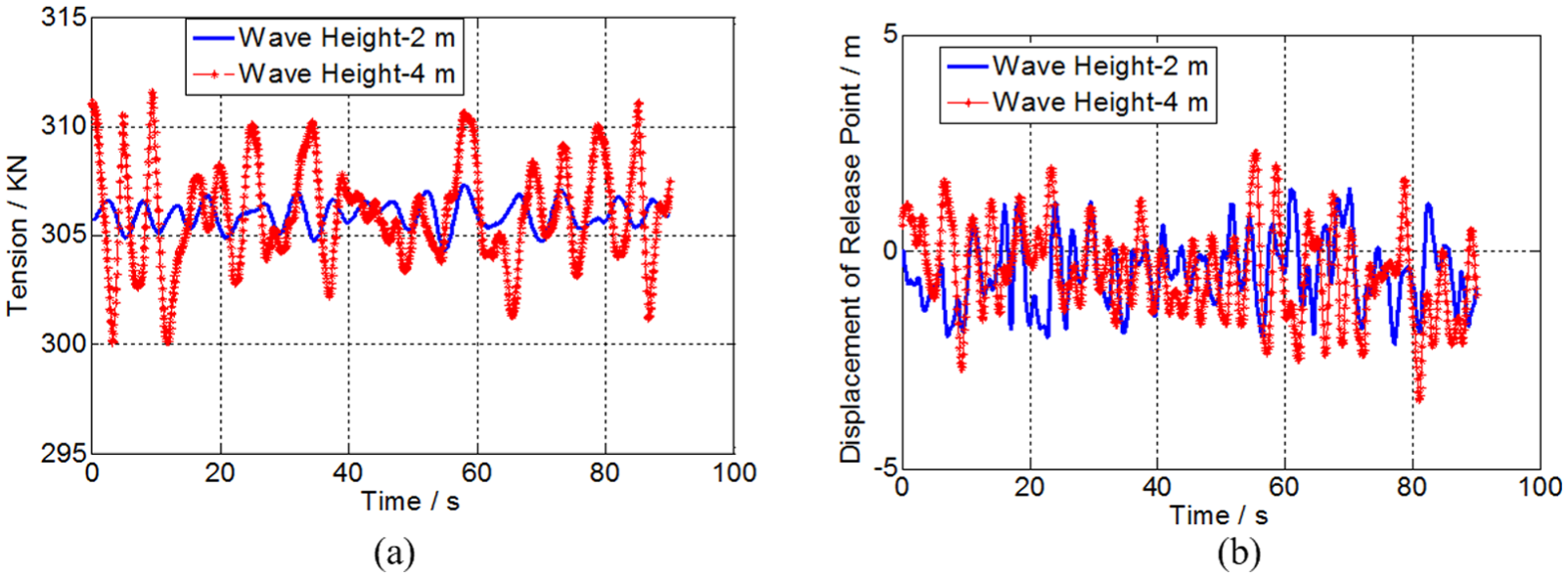
Tension and lateral vibration displacement of pipeline, L = 1200 m: (a) the tension of the pipeline root, L = 1200 m and (b) the lateral displacement at the separation point, L = 1200 m.

If the pipe-laying length is 200 m, the maximum lateral vibration amplitude (displacement) is 1.25 m when the wave height is 2.0 m, and the lateral vibration amplitude reduces to 0 m at point of 100 m; the maximum lateral vibration amplitude is 1.9 m when the wave height is 4.0 m, and the lateral vibration amplitude reduced to 0 m at the point of 170 m. If the pipe-laying length is 1200 m, the maximum lateral vibration amplitude is 1.4 m when the wave height is 2.0 m, and the lateral vibration amplitude reduces to 0 m at point of 250 m; the maximum lateral vibration amplitude is 1.6 m when the wave height is 4.0 m, and the lateral vibration amplitude reduces to 0 m at the point of 400 m.

Figure 23 shows the wave effects on the tension at the root of the pipeline and the lateral displacement at the separation point when the pipe-laying length is 1200 m. The separation point of the pipeline is the point where the pipeline loses the jacket support.

Figure 23 shows that the tension amplitude increases from 308 to 312 kN when the wave height increases from 2.0 to 4.0 m and the amplitude of the lateral displacement at the separation point increases from 2.0 to 2.6 m, which is because of the increase of the ship movement.

Conclusion

The dynamic model of the pipe-laying system is established based on the actual operating data of “Offshore Oil 201” pipe-laying ship. The deep-water pipe-laying interactive simulation system was established using semi-physical simulation technology and VR technology. In the initial pipe-laying process, the stress equation of the pipeline and cable cannot be solved due to the difficulty in defining the boundary conditions and the iterative quasi-Newton method being used:

The current will change the pipe and cable shape during the initial piping process, and the deflection is more considerable when the pipe-laying length increases. When the pipe end touches the seabed, the pipeline maximum deviation is 40 m when the current velocity increases from 0 to 2 m/s. The shape of the pipe is much more affected by the current load than the cable.

During the initial pipe laying, the current load strongly affects the pipeline tension and the tension increases from 305 to 365 kN when the current velocity increases from 0 to 2.0 m/s. The down-flow will reduce the bending moment of the pipeline. The pipe-laying operation should be designed with regard to the current load. If the current direction changes, the pipe-laying operation needs to be adjusted accordingly.

When the pipe-laying length is 200 m, the attenuation distance of the transverse vibration increases from 100 to 170 m when the wave height increases from 2 to 4 m, and when the length of pipeline is 1200 m, the attenuation distance of transverse vibration increases from 250 to 400 m. When the pipe-laying length is 1200 m and the wave height increases from 2 to 4 m, the pipeline tension will increase from 308 to 312 kN, and the vibration amplitude at the separation point will increase from 2.0 m to 2.6 m.

The technology of real-time solution for the multi-channel mathematical model, the technology of data transmission and synchronization for large data volumes of different types, and the semi-physical VR technology are the big advantages of this simulation system. The simulation system can predict the pipeline and cable real-time dynamic response in the initial pipe-laying process. The simulation system can be used not only for the rehearsal of initial pipe laying in the actual offshore project to reduce risk but also for staff training on the land.

Footnotes

Acknowledgements

The authors would like to express their gratitude to all the friends in their scientific team, who have always been helping and supporting them without a word of complaint.

Handling Editor: Jose Antonio Tenreiro Machado

Declaration of conflicting interests

The author(s) declared no potential conflicts of interest with respect to the research, authorship, and/or publication of this article.

Funding

The author(s) disclosed receipt of the following financial support for the research, authorship, and/or publication of this article: This work was supported by a grant from the National Science and Technology Major Project of China (grant no. Z12SJENA0014).

ORCID iD

Xiujun Xu

References

Grady

Harte

Localised assessment of pipeline integrity during ultra-deep S-lay installation. Ocean Eng 2013; 68: 27–37.

West

Armstrong

Mcmillan

et al . S-Lay installation of riser fairings for the independence hub. In: Paper presented at the ASME 2007 international conference on offshore mechanics and arctic engineering, San Diego, CA, 10–15 June 2007. New York: ASME.

Öner

AA.

Numerical investigation of flow around a pipeline with a spoiler near a rigid bed. Adv Mech Eng. Epub ahead of print 2 June 2016. DOI: 10.1177/1687814016651794.

How

BVE

et al . Robust adaptive boundary control of a flexible marine riser with vessel dynamics. Automatica 2011; 47: 722–732.

Zhi-Gang

Cong

Ning

et al . An overview of deepwater pipeline laying technology. China Ocean Eng 2008; 22: 521–532.

Kang

Zhang

Analysis of operability envelopes for pipe laying of deepwater steel catenary risers. J Harbin Eng Univers 2016; 37: 110–115, 122.

Lin

Gong

Jin

et al . Analysis on buckling performance of submarine pipelines during deepwater pipe-laying operation. China Ocean Eng 2009; 23: 303–316.

Shah

Mehta

Katre

A review of new technologies: AR, VR, MR. Int J Comput Appl 2017; 171: 40–44.

Shao

Guan

Tan

Virtual reality aided positioning of mobile C-arms for image-guided surgery. Adv Mech Eng. Epub ahead of print 15 February 2015. DOI: 10.1155/2014/943025.

10.

Liu

Virtual reality method of portal slewing crane based on WPF. Adv Mech Eng. Epub ahead of print 27 January 2015. DOI: 10.1155/2013/320757.

11.

Schultheis

Rizzo

AA.

The application of virtual reality technology in rehabilitation. Rehabil Psychol 2001; 46: 296–311.

12.

H-F

Xing

Zhang

Application of virtual reality technology in scenery simulation system. Comput Eng Des 2006; 27: 1108–1110.

13.

Gao

Huang

et al . Designing and implementing of a missile’s visual simulation system based on OpenGL. Acta Armamentarii 2007; 28: 125–128.

14.

Ouakad

Al-Qahtani

Hawwa

MA.

Influence of squeeze-film damping on the dynamic behavior of a curved micro-beam. Adv Mech Eng. Epub ahead of print 13 June 2016. DOI: 10.1177/1687814016650120.

15.

Abbas

Rui

Free vibration characteristic of multilevel beam based on transfer matrix method of linear multibody systems. Adv Mech Eng. Epub ahead of print 14 February 2014. DOI: 10.1155/2014/792478.

16.

Aragón Artacho

Belyakov

Dontchev

AL.

Quasi-Newton method. Investigació 2013.

17.

Byrd

Hansen

Nocedal

et al . A stochastic quasi-Newton method for large-scale optimization. SIAM J Optimiz 2015; 26: 1008–1031.

18.

Zhang

Wang

XJ.

The application of OFFPIPE in pipelaying calculation. China Offshore Platf 2014; 29: 52–56.

19.

Gan

Research on 3DMax models optimizing display in skyline spherical space. Geosp Inf 2016; 14: 7–10.

20.

Novak

Kobrehel

et al . Conformational behaviour of 11-O-methylazithromycin in the solid and solution state. Croat Chem Acta 2001; 74: 327–341.

21.

Hantoro

Utama

IKAP

Erwandi

SA.

Unsteady load analysis on a vertical axis ocean current turbine. Gastroenterology 2009; 144: S-1111.

22.

Araújo

MDV

Neto

SRDF

Lima

AGBD

et al . Hydrodynamic study of oil leakage in pipeline via CFD. Adv Mech Eng. Epub ahead of print 12 February 2015. DOI: 10.1155/2014/170178.

23.

Komatsu

Yoshida

Watanabe

et al . Degradation behavior of anode-supported solid oxide fuel cell using LNF cathode as function of current load. J Power Sources 2010; 195: 5601–5605.

24.

Zhao

F-X

Zhan

SY.

Modeling and simulation of shallow ocean wave based on small amplitude wave theory. J Syst Simul 2008; 20: 281–284.

25.

Tarp-Johansen

NJ.

Partial safety factors and characteristic values for combined extreme wind and wave load effects. J Sol Energ: T ASME 2005; 127: 242–252.

26.

Chen

Niu

et al . Direct solution of MoM matrix equation using Sherman-Morrison-Woodbury formula-based algorithm with ACA-SVD. In: Paper presented at the microwave conference, Nanjing, China, 6–9 December 2015. New York: IEEE.

27.

Sun

DZ.

Present situation and future progression of coordinate standard of architatural madule. J Gansu Univers Technol 2002; 23: 100–103.

28.

Aldraihem

Wetherhold

Singh

Intelligent beam structures: Timoshenko theory vs. Euler-Bernoulli theory. In: IEEE international conference on control applications, Dearborn, MI, 15 September–18 November 1996, pp.976–981. New York: IEEE.

29.

Murty

AVK

. Toward a consistent beam theory. AIAA J 2015; 22: 811–816.

30.

Rashidifar

Ahmadi

Vibration analysis of randomly oriented carbon nanotube based on FGM beam using Timoshenko theory. Adv Mech Eng. Epub ahead of print 2 November 2014. DOI: 10.1155/2014/653950.

31.

Akbari

Ganji

Goltabar

AR.

Dynamic vibration analysis for non-linear partial differential equation of the beam-columns with shear deformation and rotary inertia by AGM. Dev Appl Ocean Eng 2014; 3: 22–31.

32.

Ramos

Covas

Borga

et al . Surge damping analysis in pipe systems: modelling and experiments. J Hydraul Res 2004; 42: 413–425.

33.

Gobat

Grosenbaugh

MA.

Time-domain numerical simulation of ocean cable structures. Ocean Eng 2006; 33: 1373–1400.

34.

Bai

Zhao

DY.

Computer aided optimization technology based on OFFPIPE for offshore pipeline S-lay design. Pet Eng Constr 2011; 37: 14–22.

Modeling of submarine initial pipe-laying process and its real-time semi-physical virtual reality system

Abstract

Keywords

Introduction

Interactive simulation system for deep-water pipe laying

Pipe-laying operation system

Pipe-laying simulation system

Establishment of virtual environment

Mathematical model of initial pipe laying

Ship motion system modeling

Mathematical model of the environmental load

Current load

Wave load

Pipeline mathematical model

Static force analysis of the pipeline

Vibration of the pipeline

Stress analysis of the cable

Numerical algorithm

Discrete differential equation

Numerical solution of equations

Simulation cases and analysis

Initial pipe-laying process

Comparison and verification

Current load and wave effects

Current load effects

Wave effects

Conclusion

Footnotes

Acknowledgements

Declaration of conflicting interests

Funding

ORCID iD

References