Adhesion state estimation based on improved tire brush model

Abstract

On the basis of calculating the longitudinal force using the original brush model, we simplify the tire structure and consider the lateral force generated by the lateral elasticity of the tread. At the same time, the boundary conditions between the adhesion area and the slip zone in the contact area of the tire are fully discussed. By establishing an improved tire brush model, the error caused by neglecting the sideslip characteristics is avoided, and the adaptability of the tire model is improved. A double nonlinear compensation method based on the lateral acceleration deviation and the yaw rate deviation is employed to estimate the road adhesion coefficient, which is closer to the actual attachment situation than the standard calculation. Based on this model, the vehicle stability coefficient k is defined and calculated to describe the stability of the vehicle during the driving process. The modeling results show that the value of k is always in the stable range of [0, 1]. Therefore, the vehicle that utilizes the improved tire brush model is always within the controllable range in the driving process, which verifies the effectiveness of the model.

Introduction

The most important part of the vehicle in contact with the road is the tire. Through the tire, a vehicle can control the vertical, longitudinal and horizontal forces it experiences. ¹ Therefore, an accurate identification of the road surface’s attachment coefficient is a necessary condition to properly observe the tire force. Therefore, it is particularly important to select an appropriate tire model in order to obtain more accurate information on the state of the vehicle.

Researchers have achieved great progress in establishing an accurate tire model.^2–9 There are two kinds of tire model, which are the empirical model and the physical model. The empirical model is based on existing tire test data, which is manipulated through interpolation or the function-fitting method to create a formula that can predict a tire’s characteristics, such as the power index unified tire model,^2,3“magic formula” tire model,^4,5 SWIFT tire model, and Dugoff tire model. Physical models, however, mainly use a string model, brush model, beam model, spoke model, and so on.^6,7 Empirical models require a lot of experimental data and cannot intuitively reflect a tire’s complex mechanical properties. The physical model, however, has a simple structure and can directly reflect the interaction between the tire and the road with good adaptability. In the physical tire model, the tire is normally simplified to a radial elastic element, which is ideal, easily solved using physical knowledge and not restricted by other factors. The “brush model” is one such physical model, which assumes a rigid carcass and ignores the force produced by contact deformation between the tread rubber and the surface of the ground. The model then analyzes the longitudinal force of the tire according to the elastic deformation of each elastic element. ¹⁰ Zhao et al. ¹¹ took the difference in stiffness between the tire tread and the tire shoulder into consideration, and introduced a modified vertical stiffness and longitudinal stiffness, which were used to establish a modified tire brush model. However, in reality, a car in motion is often undergoing different degrees of acceleration and braking. Under actual driving conditions, the road surface exerts both longitudinal and lateral forces on the tire. ¹² Liu et al.^13–15 considered the effect of the tire tread’s lateral elasticity, but they have not yet considered it in combination with the longitudinal force.

The pavement’s adhesion coefficient is used to characterize the maximum friction potential between the tires and the pavement. Many scholars have done a lot of research work in this field. Researchers^16,17 have divided the pavement adhesion coefficient estimation method into effect-based and cause-based methods. The road surface’s adhesion coefficient is estimated using various mechanical parameters that are part of the process of automobile driving/braking. Specifically, the recognized method of estimating the adhesion’s rate of change is based on using the slope of a μ–S and a formula-fitting method.

V Jorge et al. ¹⁸ and R Rajamani et al. ¹⁹ estimated the longitudinal stiffness (the slope of the μ–S) of the μ–S curve to determine the adhesion coefficient using the method of least squares and the Kalman filter.

The tire brush model assumes that the tire’s elastic tread is a series of elastic bristles that can be stretched out on a rigid base (the wheel hub). These bristles bear the vertical load as well as the longitudinal and lateral components of the frictional forces acting on the wheel. The interaction between the tire and the road surface can be obtained by integrating the resultant forces acting on the bristles in the contact area between the tread and the ground. Thus, the adhesion characteristics of the car can be studied intuitively by combining the adhesion model with the tire brush model.^10,11 In this article, an improved tire brush model is selected, which takes both the longitudinal deformation of the tire and the lateral displacement caused by the addition of cornering characteristics into consideration. The boundary conditions for the attachment zone and the slip zone within the contact zone between the tire and the road surface are studied. The method chosen to estimate the road adhesion coefficient in this article is a double nonlinear compensation based on both the lateral acceleration deviation and the yaw rate deviation. Finally, to characterize the stability of the vehicle during driving conditions, the vehicle stability factor k is both defined and tested in double-lane change circumstances. The stability of the vehicle is judged by the data obtained from the test. These data will then be used to improve the handling and stability of the vehicle.

The theory of the improved tire brush model

According to the brush tire model, the tire tread is assumed to be rigid, and the force is produced by the contact deformation between the tire tread’s rubber and the ground. A top and side view of the established model can be seen in Figures 1 and 2.

Figure 1.

Contact deformation of tire and ground in side view.

Figure 2.

Brush model moving station in top view.

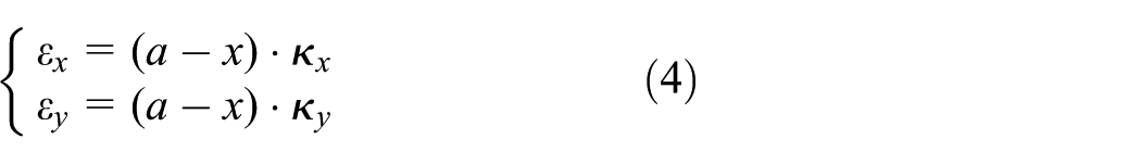
The contact length between the tire and the ground is 2a. Take the brush unit, and in the combined slip condition, the deformation of the brush ²⁰ unit is

$$\{\begin{array}{c}{\epsilon }_x=-(v_{x}t-\omega rt)\\ {\epsilon }_y=-v_{y}t\end{array}$$

(1)

Let $(a-x)=\omega \mathrm{rt}$ , then formula (1) can be converted into

$$\{\begin{array}{c}{\epsilon }_x=(a-x)·\frac{\omega r-v_x}{\omega r}\\ {\epsilon }_y=(a-x)·\frac{-v_y}{\omega r}\end{array}$$

(2)

Obviously, the longitudinal slip ratio can be written as $s=-v_x-\omega r/v_x$ , so we can define the theoretical slip as

$$\{\begin{array}{c}{\kappa }_x=-\frac{v_x-\omega r}{\omega r}\\ {\kappa }_y=\frac{-v_y}{\omega r}=({\kappa }_x-1)·\tan \delta \end{array}$$

(3)

Then, formula (2) can be written as

$$\{\begin{array}{c}{\epsilon }_x=(a-x)·{\kappa }_x\\ {\epsilon }_y=(a-x)·{\kappa }_y\end{array}$$

(4)

The local horizontal contact force acting on the brush unit can be written as

$$\{\begin{array}{c}{F}_{ax}=C_{ax}{\epsilon }_x=C_{ax}(a-x)·{\kappa }_x\\ F_{ay}=C_{ay}{\epsilon }_y=C_{ay}(a-x)·{\kappa }_y\end{array}$$

(5)

where $C_{\mathrm{ax}}$ and $C_{\mathrm{ay}}$ are the brush unit stiffness in the longitudinal and slip direction, respectively.

Due to the restriction of the road adhesion conditions, the longitudinal force of the tire will not further increase with the increasing slip ratio when the tire is at the adhesion limit. Therefore, there is a boundary point b between the adhesion zone and the slip zone in the contact area. When $x\in (-a,b)$ , the tire is in the slip zone. Conversely, when $x\in (b,a)$ , the tire is in the adhesion zone, as shown in Figure 2. Assuming that the distribution of the vertical force per unit length of the tire is symmetric and parabolic, the following holds ²¹

$$q_z\left(x\right)=\frac{3F_z}{4a}\left[1-{\left(\frac{x}{a}\right)}^2\right]$$

(6)

The vertical force of the brush unit $F_{\mathrm{az}}(x)$ is

$$F_{az}\left(x\right)=q_z\left(x\right)$$

(7)

If the road adhesion coefficient is $\mu$ , the horizontal force of each unit for brush is

$$F_a\left(x\right)\le \mu F_{az}\left(x\right)$$

(8)

where $\mu =\sqrt{{\mu }_x^2+{\mu }_y^2}$ and $F_a=\sqrt{F_{\mathrm{ax}}^2+F_{\mathrm{ay}}^2}$ .

At the boundary point b, the horizontal force reaches its maximum, which means that $F_a(b)=\mu F_{\mathrm{az}}(b)$ . Combining with formulas (5)–(7), we get

$$\sqrt{F_{\mathrm{ax}}{(b)}^2+F_{\mathrm{ay}}{(b)}^2}=\frac{3\mu F_z}{4a}[1-{\left(\frac{b}{a}\right)}^2]$$

(9)

therefore, $b=(4a^{3}A/3\mu F_Z)-a$ , where $A=\sqrt{C_{\mathrm{ax}}^2{\kappa }_x^2+C_{\mathrm{ay}}^2{\kappa }_y^2}$ .

According to the above theory on the force per brush unit, the total longitudinal and lateral force on the tire in the contact area can be expressed as

$$\{\begin{array}{c}{F}_x=\underset{-a}{\overset{b}{\int }}{\mu }_x{q}_z\left(x\right)\mathrm{dx}+\underset{b}{\overset{a}{\int }}{F}_{\mathrm{ax}}\left(x\right)\mathrm{dx}\hfill \\ \multicolumn{1}{c}{F_y=\underset{-a}{\overset{b}{\int }}{\mu }_y{q}_z\left(x\right)\mathrm{dx}+\underset{b}{\overset{a}{\int }}{F}_{\mathrm{ay}}\left(x\right)\mathrm{dx}}\end{array}$$

(10)

We then obtain

$$\{\begin{array}{c}\multicolumn{1}{c}{F_x=\frac{{\mu }_x{F}_z}{4a^3}(a^3+3a^{2}b-b^3)+}\\ C_x·{\kappa }_x·(\frac{1}{2}{a}^2+\frac{1}{2}{b}^2-\mathrm{ab})\hfill \\ \multicolumn{1}{c}{F_y=\frac{{\mu }_y{F}_z}{4a^3}(a^3+3a^{2}b-b^3)+}\\ C_y·{\kappa }_y·(\frac{1}{2}{a}^2+\frac{1}{2}{b}^2-\mathrm{ab})\hfill \end{array}$$

(11)

where $C_x,C_y$ are the longitudinal and lateral stiffness of the tread elements, and $C_{x/y}=2a^2{C}_{\mathrm{ax}/\mathrm{ay}}$ .

The definition of steady state

The establishment of the vehicle dynamic model

Considering the longitudinal motion along the x-axis, the lateral movement along the y-axis, and the yaw motion along the z-axis, we establish a nonlinear vehicle model with three coupled degrees of freedom, including the yaw, lateral, and longitudinal directions, as shown in Figure 3

$$\begin{array}{c}\multicolumn{1}{c}{a_x=\frac{(F_{y1}+F_{y2})\sin \delta }{m}+\frac{F_{x3}+F_{x4}}{m}}\\ \multicolumn{1}{c}{+\frac{(F_{x1}+F_{x2})\cos \delta }{m}}\end{array}$$

(12)

$$\begin{array}{c}\multicolumn{1}{c}{a_y=\frac{(F_{x1}+F_{x2})\sin \delta }{m}+\frac{F_{y3}+F_{y4}}{m}}\\ \multicolumn{1}{c}{+\frac{(F_{y1}+F_{y2})\cos \delta }{m}}\end{array}$$

(13)

$$\begin{array}{c}\multicolumn{1}{c}{\stackrel{·}{\omega }=[(F_{y1}+F_{y2})\cos \delta ·L_a}\\ \multicolumn{1}{c}{+(F_{x1}+F_{x2})\sin \delta ·L_a-(F_{y3}+F_{y4})}\\ \multicolumn{1}{c}{·L_b+(F_{y1}-F_{y2})\sin \delta +(F_{x2}-F_{x1})}\\ \multicolumn{1}{c}{\cos \delta ·L_c+(F_{x4}-F_{x3})·L_c]/I_z}\end{array}$$

(14)

where m is the total mass of vehicle; $I_z$ is the moment of inertia of vehicle around the vertical z-axis; $\delta$ is the front steering wheel angle; $a_x,a_y$ is the longitudinal and lateral acceleration at the centroid, respectively; $\beta$ is the sideslip angle of the centroid; r is the yaw angular speed; $L_a,L_b$ is the distance from the centroid to the front or the rear axle; and $L_c$ is the length of half of the wheelbase.

Figure 3.

Vehicle model of 3 degrees of freedom.

The definition of vehicle stability factor

Li et al. ²² divided the vehicle’s driving state into a stable region, a less stable region, a critical region of instability and an unstable region. The vehicle stability factor k can be defined as

$$k=\frac{a_y}{\mu g}$$

(15)

where $a_y$ is the lateral acceleration, g is the acceleration of gravity, and $\mu$ is the road adhesion coefficient. The vehicle stability coefficient is the key factor that represents the stability of the vehicle while it is being driven. When $k<0.5$ , the car is in a stable region; when $0.5<k<0.75$ , the car is in a less stable region; when $0.75<k<1$ , the car is in the critical region of instability; and when $k>1$ , the car is in a unstable region and is out of control. Therefore, a vehicle can be driven safely, if the stable coefficient of the vehicle is less than 1 at any given time. Current electronic stability systems integrate the safety control systems such as braking, accelerating, steering, and so on. When a vehicle is in the less stable region where $0.5<k<0.75$ , the electronic stability system begin to control the vehicle back into the stable region. This means that the vehicle stability coefficient k has a significance that merits study, as it can accurately judge the stability of a vehicle at a certain point in time through the value k. Furthermore, electronic stability systems use k to control the vehicle’s stability.

Road adhesion coefficient estimation

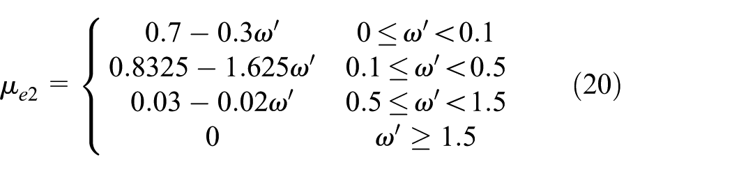
Chen et al. ²³ and Li et al. ²⁴ put forward an algorithm to estimate the road adhesion coefficient using double nonlinear compensation based on the lateral acceleration deviation and the yaw rate deviation

$$\mu =\left|G_y\right|+{\mu }_e=\frac{a_y}{g}+{\mu }_e$$

(16)

where ${\mu }_e$ is the estimation deviation compensation.

Nonlinear compensation based on $a_y$ is sensitive to oversteer, which is rectified by

$$a\prime =|v_x·\omega -a_y|$$

(17)

where $a\prime$ is the nonlinear compensation based on $a_y$ .

Based on the fact that $\omega$ is sensitive to understeer, $\omega \prime$ is the nonlinear compensation based on $\omega$

$$\omega \prime =|{\omega }_r-\omega |=|\frac{{\omega }_{r\_s}}{1+\mathrm{Ts}}-\omega |$$

(18)

where ${\omega }_{r\_s}$ is the yaw response of steering steady, ${\omega }_{r\_s}=(v_x/L)/(1+K{v_x}^2)\delta$ , K is the stability factor, T is the lag time coefficient, and s is the Laplace operator.

The deviation compensation estimations are designed as follows

$${\mu }_{e1}=\{\begin{array}{cc}0.7-0.667a\prime \hfill & 0\le a\prime <0.15\hfill \\ \multicolumn{1}{c}{1.13-3.533a\prime }& 0.15\le a\prime <0.3\hfill \\ \multicolumn{1}{c}{0.112-0.14a\prime }& 0.3\le a\prime <0.8\hfill \\ \multicolumn{1}{c}{0}& a\prime \ge 0.8\hfill \end{array}$$

(19)

$${\mu }_{e2}=\{\begin{array}{cc}0.7-0.3\omega \prime \hfill & 0\le \omega \prime <0.1\hfill \\ \multicolumn{1}{c}{0.8325-1.625\omega \prime }& 0.1\le \omega \prime <0.5\hfill \\ \multicolumn{1}{c}{0.03-0.02\omega \prime }& 0.5\le \omega \prime <1.5\hfill \\ \multicolumn{1}{c}{0}& \omega \prime \ge 1.5\hfill \end{array}$$

(20)

$${\mu }_e=({\mu }_{e1}<{\mu }_{e2}):{\mu }_{e1}:{\mu }_{e2}$$

(21)

From formula (21), we choose the smaller values for the deviation compensation estimation.

Vehicle test verification

To verify the accuracy and timeliness of the above proposed theoretical model, we choose a vehicle with a 215/75R17.5 tire model to test in double-lane road conditions, as shown in Figure 4. The purpose of this test is to record the variation range of the vehicle stability factor k and judge the stability of the vehicle while driving in simulated conditions through the curves of value k.

Figure 4.

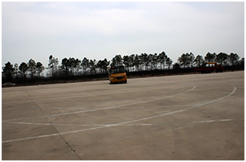
Real vehicle test.

A diagram of the double-lane road test is shown in Figure 5. The vehicle runs along the path shown at a constant speed 80 km/h.

Figure 5.

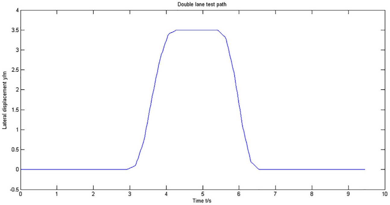
Double-lane test path.

The parameters of the test vehicle are shown in Table 1.

Table 1.

Test vehicle parameters.

Parameter name	Dimension	Value
The total height of no-load vehicle	mm	2880
The distance from the centroid to the front axle	mm	4291
The distance from the centroid to the rear axle	mm	2806
Front track	mm	1847
Rear track	mm	1650
The total mass of no-load vehicle	kg	5240
Moment of inertia around the z-axis	kg m2	12,300
Front effective cornering stiffness, k1	N/rad	−1.521 × 105
Rear effective cornering stiffness, k2	N/rad	−3.022 × 105
Tire model	none	215/75R17.5

The vehicle’s speed during the experiment is shown in Figure 6, which is controlled to be 80 km/h. There is a small variation in the speed from 80 km/h during the test.

Figure 6.

Vehicle speed over time.

The longitudinal, lateral, and vertical force of the tire generated by the vehicle in double-lane change path is shown in Figures 7–9.

Figure 7.

The changes in longitudinal force.

Figure 8.

The changes in lateral force.

Figure 9.

The changes in vertical force.

Figure 7 shows the changes in the tire’s longitudinal force. The force of the front wheel is zero because a rear-wheel drive vehicle was used in this test. Between 0 and 0.3 s, vehicle’s speed is significantly reduced, and the longitudinal acceleration is less than zero. Therefore, the tire’s force is initially acting in the negative direction. However, the speed increases back to nearly 80 km/h almost immediately, and the longitudinal force similarly increases to nearly 250 N. Near the 3-s mark, the vehicle starts to turn left, the speed decreases slightly, and the longitudinal force is appropriately smaller. During the double-lane portion of the test, the longitudinal force oscillates near 200 N.

As shown in Figure 8, when the vehicle is traveling in a straight line during the first 2 s, the lateral force is zero. Near the 3-s mark, the vehicle turns left and the lateral force gradually increases to a peak and then begins to decrease. Near the 4-s mark, the vehicle turns right, which causes the lateral force to become more negative as time progresses. At 5.5 s, the lateral force caused when the vehicle turns left for the second time is larger than it was during the first left turn due to both the previous two right turns and due to inertia. Furthermore, because of the vehicle’s right turn, the lateral force on the left side of the vehicle is larger than that on the right side. After 6.5 s, the vehicle continues to turn left, and the lateral force becomes larger with an increase in time, which is slightly higher on the right side of the vehicle than that on the left side due to the left turn.

As shown in Figure 9, due to the distribution of the vertical axial load, the front and rear wheels initially experience different vertical forces. When vehicle turns left, the vertical forces in the left wheels decrease and increase gradually in the right wheels, Furthermore, the force is distributed symmetrically because the roll leads the body camber. The opposite effect can be seen when the vehicle turns right.

Figure 10 shows for the calculated adhesion coefficient as a function of time. The solid line represents the estimation results using the double nonlinear compensation method, and the dashed line represents the results from the conventional calculation, which is the ratio of horizontal force and vertical force on the tire.

Figure 10.

The changes in the adhesion coefficient with time.

The test pavement is a dry cement surface, and the adhesion coefficient ranges from 0.8 to 0.9. Within the first 2 s, the vehicle drives in a straight line, and the adhesion coefficient should be close to the theoretical value. However, the lateral force at that time is zero, and the adhesion coefficient calculated is therefore also zero. Obviously, the estimated results obtained using double nonlinear compensation are closer to the actual adhesion coefficient. When the vehicle turns, the vehicle is in a dynamic steady state. The adhesion coefficient decreases accordingly and fluctuates when compared to the initial steady state. Finally, the vehicle returns to a stable state, and the adhesion coefficient returns to 0.8–0.9.

Figure 11 is a graph showing the variation of the vehicle stability factor k with time, from which we can see that the value is in the range between 0 and 1. Between 0 and 2 s, the vehicle is driving straight without any lateral force, and the value of k is zero when vehicle is in a stable and safe condition. The vehicle begins to turn left at the 3-s mark. The value of k increases gradually with the lateral force, and the driving state becomes more and more unstable, moving from the stable region to the critical region of instability. At its peak, the value of k is near 0.9, which is in the critical region of instability. In the conventional calculation, there are two low points in the value of k at 4 s and 6 s, which are caused by lateral forces acting in opposite directions. During the left turn, the lateral force is positive (directed to the right), and during the right turn, the lateral force is negative (directed to the left). The corresponding reduction in the numerical value of the lateral force does lead to a low point in k. However, in actuality, the vehicle’s state at these points remains unstable, and the original method has some degree of bias. After 8 s, the vehicle returns to a more stable state.

Figure 11.

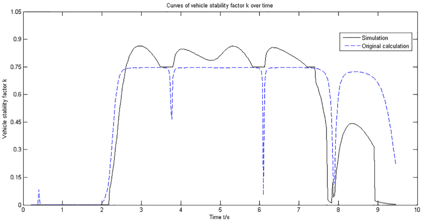
The changes in k with time.

At a certain speed and when the vehicle is traveling in a straight line, the value of k is zero and remains unchanged, and when the vehicle turns a certain angle, a change in the value of k ensues that is proportional to the changes of the tire’s angle. Thus, it can be concluded that k is almost unaffected by the speed but is related to steering. This is also in line with the actual running condition of the vehicle. The vehicle is more stable when it drives in a straight line and has relatively poor stability when steering.

During the entirety of the double-lane test, the vehicle does not exceed the boundaries of instability and is always within the range of critical instability. It can control the vehicle back to a stable driving state by the dynamics stability control system to a certain extent. Therefore, the driving parameters can be effectively estimated using the corrections to the adhesion coefficient in combination with the theoretical improved tire brush model presented in this work.

Conclusion

1. In this article, we simplify the structure of the tire and deduce formulas for the tire’s longitudinal and lateral forces according to the deformation of the tread unit. The boundary conditions between the attachment zone and the slip zone within the contact area are also discussed.

2. We choose to use a double nonlinear compensation method based on the lateral acceleration deviation and the yaw rate deviation to estimate the road adhesion coefficient. Comparing the estimation to the conventional calculation, we see that the double nonlinear compensation method better reflects the real-world conditions.

3. To mathematically characterize the vehicle’s stability during operation, we define the vehicle stability factor k. The results indicate that the value of the vehicle stability factor k changes when the vehicle turns at certain speeds, and when traveling in a straight line, k is always zero. These observations are in line with the fact that steering can cause instability during when driving at certain speeds. The value of k obtained from the test is within the range of [0, 1], and the vehicle stays within the controllable range for the entire test. This verifies that the vehicle using the above mentioned theory is relatively stable in actual driving conditions. The theory and method mentioned above are both effective and feasible.