Thermal analysis of an electromagnetic linear actuator

Abstract

This article presents a new electromagnetic linear actuator applied in the electromagnetic-driven valve train. To clarify the actuator’s temperature rise and heat distribution, a heat transfer model was established by analyzing the complex heat exchange inside the actuator theoretically. A two-way coupling finite model of the electromagnetic linear actuator was built up, and the simulation calculation was carried out based on Ansoft Maxwell and ANSYS Workbench. In order to verify the accuracy of the theoretical analysis and simulation model, the temperature rise was tested. Comparing the data of test and simulation, results show that the error is controlled well within 6.54%. Finally, laws of the electromagnetic linear actuator’s temperature rise and distribution were analyzed, which would lay a solid foundation for follow-up research on the cooling and heat dissipation of the electromagnetic linear actuator.

Introduction

The electromagnetic-driven valve train (EDVT), as an important form for camless valve train, has attracted more and more attention in academic studies at home and abroad. Compared with traditional cam valve train and mechanical variable valve train, the adoption of the EDVT will effectively reduce fuel consumption and improve engine efficiency and fuel economy.^1–5

The electromagnetic linear actuator (ELA) applied in the EDVT is tubular moving-coil linear motor. Then, it is called actuator to highlight its characteristics as the actuator of motion control which is different from the normal linear motors with relatively low performance evaluation or a power application. Compared with the flat or other linear motor, the tubular moving-coil linear motor has the advantages of compact structure, high linearity, and high power density.^6–10 But it has some disadvantages as well, such as high internal energy consumption, fast temperature rising, and poor heat dissipation. ¹¹

There are scarce studies on the linear motor’s energy consumption and temperature rising of the similar ELA in and abroad at present. Huang et al., ¹² from Harbin Institute of Technology, have conducted calculation and experimental analysis on tubular permanent magnet linear motor under high load and discussed the limited conditions of the motor. Tomczuk and Waindok, ¹³ from Opole University of Technology of Poland, have researched the temperature rise influence of the linear actuator they studied. The research shows that both permanent magnet’s performance parameter and maximum current density of the actuator decrease along when the temperature goes up. And then it affects the linear actuator’s performance. Whereupon, in order to lower the inner temperature of the tubular sealed linear motor and improve its performance, Wang in Beijing University of Aeronautics and Astronautics proposes using magnetic fluid to improve the thermal efficiency of the linear motor. This helps to dissipate heat in the motor’s inner core and windings by magnetic fluid, so that it lowers inner temperature of the motor. ¹⁴ Nevertheless, widespread and application of this proposal is limited due to assembly and seal difficulty, rare magnetic fluid, and high cost. Marignetti ¹⁵ from Italy tries to cool the winding coil of the tubular linear actuator using liquid nitrogen. Results show that cooling effect is significant: the winding coil’s temperature decreases about 90% through liquid nitrogen cooling. Because of its large size, complex structure, and high price, it has also faced with problems to apply in micro space and bulk industrial production.

Analyzing temperature rise and heat distribution is a study on the forms of the actuator’s energy consumption, which will provide an excellent foundation for research of the actuator’s consumption reduction, heat dissipation, and performance improvement. This article, starting from analysis of heat generation of the ELA, establishes the actuator’s heat transfer model and analyzes its temperature rise and distribution via finite element simulation calculation software. Moreover, it further verifies the accuracy and reliability of the actuator’s heat transfer model and simulation calculation by the temperature rising test.

Heat transfer modeling of the ELA

Basic structure of the ELA

The ELA researched in this article is mainly applied in the EDVT, and its basic structure is shown in Figure 1. By Halbach array of the permanent magnet, the field of the air gap in the ELA is strengthened. At the same time, the armature reaction is improved using a special electromagnetic coil arrangement so that the driving force of the actuator, which is independent of the position, is proportional to the control current. Additionally, the ELA has many advantages such as it has small movement inertia, compact structure, and high power density. It can also meet requirements of any driving force and working operation theoretically.^16–18

Figure 1.

Schematic diagram of the ELA.

Heat generation in the ELA

First law of thermodynamics can be expressed as follows: all maters in nature have a certain degree of energy. Although energy can neither be created nor destroyed, it can be transformed from one form to another or be transferred from one (or some) object to another (or some). There is no change in the total amount of the energy during the transformation and transfer. Hence, heat generated in the ELA can be explained by this law.

Heat sources of the ELA mainly come from various losses occurring in the operation. Those losses will be converted into heat to dissipate and then all parts’ temperature of the actuator will be higher accordingly. The major parts of the ELA’s energy consumption are copper loss, iron loss, and other stray losses. Figure 2 presents the classification of all kinds of energy consumption and their distribution in the actuator.

Figure 2.

Classification and distribution of the ELA’s energy consumption.

Heat transfer model of the ELA

The heat exchanging process in the ELA is rather complicated. Dai and Chang ¹¹ deeply analyze the ELA’s energy consumption structure, distribution, and changing laws. Based on the analysis in this article, the ELA’s heat is mainly from that generated by copper loss of the winding coils and iron loss of the ferromagnetic materials. Those heats mostly concentrate in the winding coils and inner core. Part of the heat will radially transfer from inside to permanent magnet, outer yoke, and cover and finally radiates into space by convective heat exchange among outer yoke, cover, and outside air. Moreover, moving coil of the ELA moves forth and back inside, and the bottom of this actuator is open, so part of the heat in the axial direction will also transfer to outside through complicated heat conduction and convection.

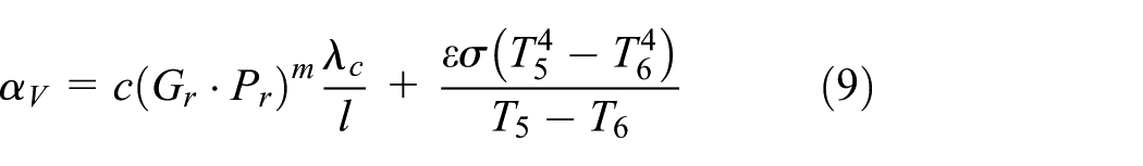
In practice, heat of the ELA transfer radiates from inner high-temperature zone to outside low-temperature zone while the path is relatively complicated. For the purpose of easy analysis, this article simplifies the ELA’s heat exchange model to radial heat transmission and axial transmission combined with the characters of the actuator’s axial symmetry.

The radial heat transfer model

Figure 3 shows the radial heat transfer model of the ELA in which area I is the inner core, area II is the moving coil, area III is the permanent magnet, area IV is the outer yoke, and area V is the outside air. Heat of areas I, III, and IV is mainly transferred by heat conduction while that of areas II and V is transferred rather complicate, especially area II. Because of the rectilinear motion of the moving coil in the ELA, there are heat conduction and comparatively heat convection existing in area II.

Figure 3.

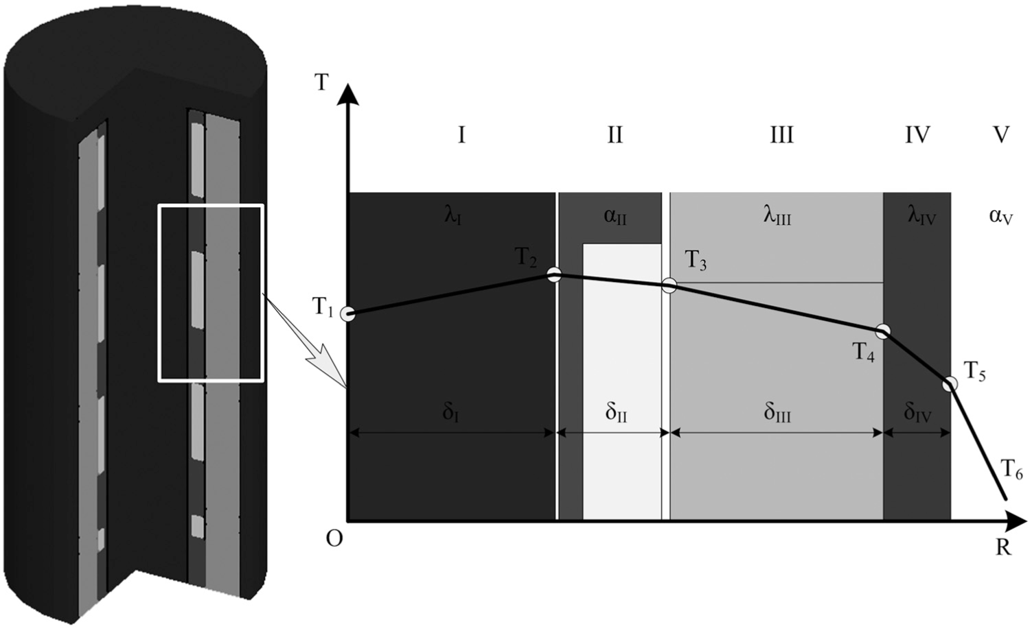
The radial heat transfer model of the ELA.

From Figure 3, we can obtain as below by the concept of overall heat transfer process

$$\{\begin{array}{c}q=\frac{{\lambda }_I}{{\delta }_I}(T_1-T_2)\hfill \\ q={\alpha }_{\mathrm{II}}(T_2-T_3)\hfill \\ q=\frac{{\lambda }_{\mathrm{III}}}{{\delta }_{\mathrm{III}}}(T_3-T_4)\hfill \\ q=\frac{{\lambda }_{\mathrm{IV}}}{{\delta }_{\mathrm{IV}}}(T_4-T_5)\hfill \\ q={\alpha }_V(T_5-T_6)\hfill \end{array}$$

(1)

Then, after compilation

$$q=\frac{Q}{A}=\frac{T_1-T_6}{\frac{{\delta }_I}{{\lambda }_I}+\frac{1}{{\alpha }_{\mathrm{II}}}+\frac{{\delta }_{\mathrm{III}}}{{\lambda }_{\mathrm{III}}}+\frac{{\delta }_{\mathrm{IV}}}{{\lambda }_{\mathrm{IV}}}+\frac{1}{{\alpha }_V}}=k_{\mathrm{total}}(T_1-T_6)$$

(2)

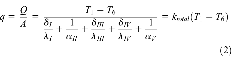
Thus, we can obtain

$$k_{\mathrm{total}}=\frac{1}{\frac{{\delta }_I}{{\lambda }_I}+\frac{1}{{\alpha }_{\mathrm{II}}}+\frac{{\delta }_{\mathrm{III}}}{{\lambda }_{\mathrm{III}}}+\frac{{\delta }_{\mathrm{IV}}}{{\lambda }_{\mathrm{IV}}}+\frac{1}{{\alpha }_V}}$$

(3)

where q is the heat flux of unit heat transfer area; Q is the total heat flux; A is the heat transfer area; $k_{\mathrm{total}}$ is the overall heat transfer coefficient; $T_1$ , $T_2$ , $T_3$ , $T_4$ , $T_5$ , and $T_6$ are interface temperatures of each area separately; ${\lambda }_I$ , ${\lambda }_{\mathrm{III}}$ , and ${\lambda }_{\mathrm{IV}}$ are heat conductivity coefficients of areas I, III, and IV, respectively; ${\delta }_I$ , ${\delta }_{\mathrm{III}}$ , and ${\delta }_{\mathrm{IV}}$ are radial thicknesses of areas I, III, and IV; and ${\alpha }_{\mathrm{II}}$ and ${\alpha }_V$ are radial heat transfer coefficients of areas II and V.

It could be found out from equation (3) that the primary factors affecting the ELA’s overall heat transfer coefficient are heat conductivity and heat transfer coefficients of each area. Heat conductivity depends primarily on the materials used in every components of the ELA, and Table 1 presents relevant attributes of those materials. Despite the heat conductivity, the critical factor impacting the overall heat transfer coefficient is the heat transfer coefficient ${\alpha }_{\mathrm{II}}$ and ${\alpha }_V$ in areas II and V.

Table 1.

Attributes of the ELA’s materials.

Materials	Property
	Density (kg/m3)	Heat conductivity (W/(m °C))		Specific heat (J/(kg °C))
Copper	8933	401		386
Aluminum	2689	222		900
NdFeB	7400	50 (25°C)		502.08
Air	1.18	5		1042
Teflon	2300	0.24		0°C	960
				50°C	1050
Steel-1008	7872	101°C	58	100°C	486
		208°C	49.2	200°C	502
		304°C	46.2	300°C	528
		405°C	43.1	400°C	556
		510°C	40	500°C	565

Area II consists of moving coil, skeleton, and air gap. There is a complex heat transfer process in a small scale, and Figure 4 shows the simplification of the model. In that, the air gap among the skeleton, inner core, and permanent magnets is much small, so the influence of the air gap on temperature gradient will be ignored to simplify the model.

Figure 4.

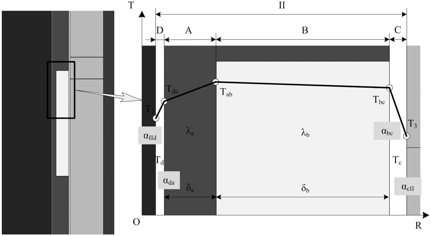
The heat transfer model in area II of the ELA.

From the overall heat transfer theory, the heat transfer coefficient ${\alpha }_{\mathrm{II}}$ in area II can be calculated as follows

$${\alpha }_{\mathrm{II}}=\frac{1}{\frac{1}{{\alpha }_{\mathrm{IId}}}+\frac{1}{{\alpha }_{\mathrm{da}}}+\frac{{\delta }_a}{{\lambda }_a}+\frac{{\delta }_b}{{\lambda }_b}+\frac{1}{{\alpha }_{\mathrm{bc}}}+\frac{1}{{\alpha }_{\mathrm{cII}}}}$$

(4)

In this equation, ${\alpha }_{\mathrm{IId}}$ , ${\alpha }_{\mathrm{da}}$ , and ${\alpha }_{\mathrm{bc}}$ are coefficients of convective heat transfer, respectively, from $T_2$ to $T_d$ , $T_{\mathrm{bc}}$ to $T_c$ , and $T_c$ to $T_3$ ; ${\delta }_a$ and ${\delta }_b$ are thicknesses of areas A and B; and ${\lambda }_a$ and ${\lambda }_b$ are heat conductivity coefficients of areas A and B, respectively.

The heat transfer method of area V, where the ELA’s outer wall contacts with the outside air, is mainly convection heat transfer and radiation as shown in equation (5)

$${\alpha }_V={\alpha }_{\mathrm{Vc}}+{\alpha }_{\mathrm{Vr}}$$

(5)

where ${\alpha }_{\mathrm{Vc}}$ is the coefficient of convective heat transfer between the ELA’s outer wall and the outside air and ${\alpha }_{\mathrm{Vr}}$ is that of thermal radiation.

Based on the natural convection heat transfer theory, the following can be obtained

$${\alpha }_{\mathrm{Vc}}=\frac{N_u{\lambda }_c}{l}=c{(G_r·P_r)}^m\frac{{\lambda }_c}{l}$$

(6)

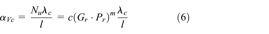
In this equation, $N_u$ , $G_r$ , $P_r$ , c, and m are numbers of Nusselt, Grashof, Prandtl, constant, and Nusselt coefficient, respectively; ${\lambda }_c$ is coefficient of air thermal conductivity at certain temperature. Since the ELA in this article is columned and vertically positioned, characteristic length l here means height of the actuator.

The thermal radiation can be derived from the Stefan–Boltzmann law

$$q=\epsilon \sigma (T_5^4-T_6^4)$$

(7)

Then

$${\alpha }_{\mathrm{Vr}}=\frac{q}{\mathrm{\Delta }T}=\frac{\epsilon \sigma (T_5^4-T_6^4)}{T_5-T_6}$$

(8)

where $\epsilon$ is object’s emissivity which is also called blackness and $\sigma$ is the Stefan–Boltzmann constant with the value of 5.67 × 10⁻⁸ W/(m² K⁴).

Finally, the coefficient of heat transfer in area V will be calculated

$${\alpha }_V=c{(G_r·P_r)}^m\frac{{\lambda }_c}{l}+\frac{\epsilon \sigma (T_5^4-T_6^4)}{T_5-T_6}$$

(9)

The axial heat transfer model

Figure 5 presents the ELA’s axial heat transfer model.

Figure 5.

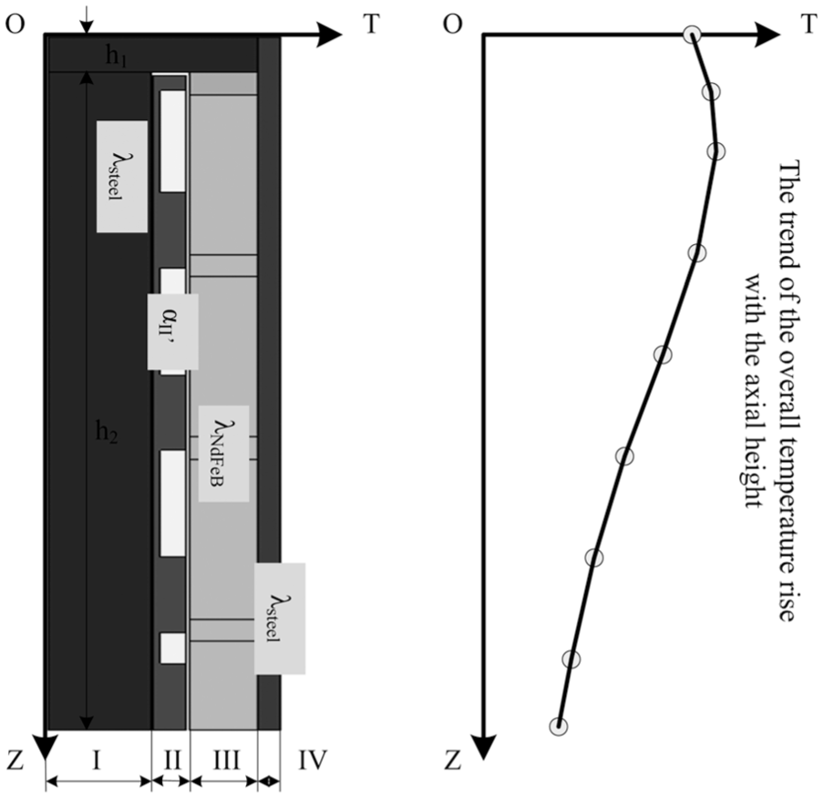
The axial heat transfer model of the ELA.

Analysis on the ELA’s axial heat transfer can be conducted from the four areas as shown in Figure 5. The heat transfer in areas I, III, and IV mostly rely on the heat conduction of the actuator’s own components while that in area II is complicate including materials’ heat conduction and heat convection caused by moving coil’s reciprocating motion. Then, the theoretical model of the ELA’s axial heat transfer could be derived according to the overall heat transfer theory in equation (10) as follows

$$\{\begin{array}{c}\alpha {\prime }_I=\frac{{\lambda }_{\mathrm{steel}}}{h_1+h_2}\left(I\right)\hfill \\ \alpha {\prime }_{\mathrm{II}}=\frac{{\lambda }_{\mathrm{steel}}}{h_1}+{\alpha }_{\mathrm{mover}}\left(\mathrm{II}\right)\hfill \\ \alpha {\prime }_{\mathrm{III}}=\frac{{\lambda }_{\mathrm{steel}}}{h_1}+\frac{{\lambda }_{\mathrm{NdFeB}}}{h_1}\left(\mathrm{III}\right)\hfill \\ \alpha {\prime }_{\mathrm{IV}}=\frac{{\lambda }_{\mathrm{steel}}}{h_1+h_2}\left(\mathrm{IV}\right)\hfill \end{array}$$

(10)

where $\alpha {\prime }_I$ , $\alpha {\prime }_{\mathrm{II}}$ , $\alpha {\prime }_{\mathrm{III}}$ , and $\alpha {\prime }_{\mathrm{IV}}$ correspond to the coefficients of axial heat transfer in areas I, II, III, and IV; ${\lambda }_{\mathrm{steel}}$ is the steel-1008 material’s coefficient of heat conduction; ${\lambda }_{\mathrm{NdFeB}}$ is the permanent magnet material NdFeB’s coefficient of heat conduction; $h_1$ is the thickness of the actuator’s cover; $h_2$ is the permanent magnet’s overall height; and ${\alpha }_{\mathrm{mover}}$ is the convective heat transfer coefficient in the moving coils and air gap.

Temperature field simulation of the ELA

In order to research more deeply on the distribution and changing laws of the ELA’s temperature field, the actuator’s model and simulation calculation could be carried out with the help of the finite element method on the basis of analysis on the ELA’s heat transfer model.

With the temperature field model of the Ansoft Maxwell and ANSYS Workbench, this article carries out coupling analysis of the electromagnetic field and temperature field which can be further divided into two forms: one-way coupling and two-way coupling. And their differences are illustrated in Figure 6.

Figure 6.

The one-way and two-way coupling models of the electromagnetic and temperature fields.

It can be seen from Figure 6 that these two coupling modes are all based on the electromagnetic field analysis, and the magnetic field mode is imported into the temperature field. Then, regarding the loss results from the magnetic field analysis as the heat source of the temperature field analysis helps to acquire the distribution and temperature rise of the ELA’s temperature field. What makes the two-way coupling different is that, analysis results of the temperature field will counter coupling to the magnetic field mode. Because of that, there will be certain adjustment in material definition of the magnetic field and setting excitation with the feedback of the temperature field result, and therefore, the simulation will be more accurate and reliable. However, there is no doubt that two-way coupling occupies more computer resources and needs longer computing time.

The ELA in this article will produce high temperature at high load working conditions which may affect the ELA’s material performance to some degree. Therefore, simulation analysis on the ELA using the two-way coupling mode of the magnetic and temperature field is more accurate and practical.

Through establishment and simulation calculation on the two-way coupling finite model of the ELA’s magnetic and temperature fields, curvilinear relation of the ELA’s simulation temperature rise could be obtained as shown in Figure 7. Moreover, to make the ELA’s temperature distribution pretty clear, Figure 8, a cloud chart of the ELA’s temperature gradient, will be gained via simulation.

Figure 7.

Curves chart of the ELA’s simulation temperature rise.

Figure 8.

Clouds chart of the ELA’s temperature distribution at different times.

Figure 7 reflects the ELA’s temperature changes at some important checkpoints while Figure 8 illustrates the ELA’s temperature distribution changing with the actuator’s running time.

Temperature rise test on the ELA

The ELA’s temperature rise test needs to be carried out in order to analyze the changing laws of the ELA’s temperature rise more practically and validate the relevant parameter of the temperature field model.

In this article, it adopts a temperature test scheme using platinum thermistor Pt100 supplemented by infrared thermal imager Fluke vt04 to test the ELA’s temperature rise under different working conditions. Figure 9 presents this testing device.

Figure 9.

Experimental installation of the ELA’s temperature rise test.

Figure 10 shows the arrangement of the platinum thermistor outside of the ELA. Since the structure of the ELA is almost axial symmetry, this temperature measuring point arrangement typically covers the actuator’s outward, beneficial to analyze and study the changing laws of the ELA’s temperature rise.

Figure 10.

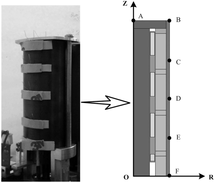
Arrangement of the platinum thermal resistance outside of the ELA.

Due to small air gap in the ELA and the moving coils’ reciprocal rectilinear motion in the actuator, it is difficult to measure the temperature rise inside the actuator especially in the moving coils. Even so, the temperature rise test inside the ELA has an important significance not only in clearing the overall heat distribution of the ELA but also in verifying the accuracy of the ELA’s temperature rise model. To deal with the problem, given that resistance $R_T$ of the ELA’s coil material, namely, copper enameled wire’s resistance $R_T$ , has relation with temperature rise $\mathrm{\Delta }T$ as shown in equation (11), the average temperature of moving coils can be calculated through precise measurement of the winding coil’s resistance

$$\mathrm{\Delta }T=\frac{R_T-R_0}{R_0}(T_0+234.5)$$

(11)

In this equation, $R_T$ and $R_0$ are, respectively, the coil’s resistances when temperatures are T and $T_0$ .

Test will be conducted without any cooling measures. For the purpose of comparison and analysis not repeated, it researches the temperature rise when the engine speed is 3000 r/min, and thus, the changing curve of temperature rise at all test points can be gained as in Figure 11. Through measurement on the winding coil’s resistance value using the precise resistance tester when the ELA breaks down, it can figure out the changing curve of the winding’s temperature inside the ELA in natural cooling as presented in Figure 12.

Figure 11.

Change curves of temperature rise at test points outside the ELA.

Figure 12.

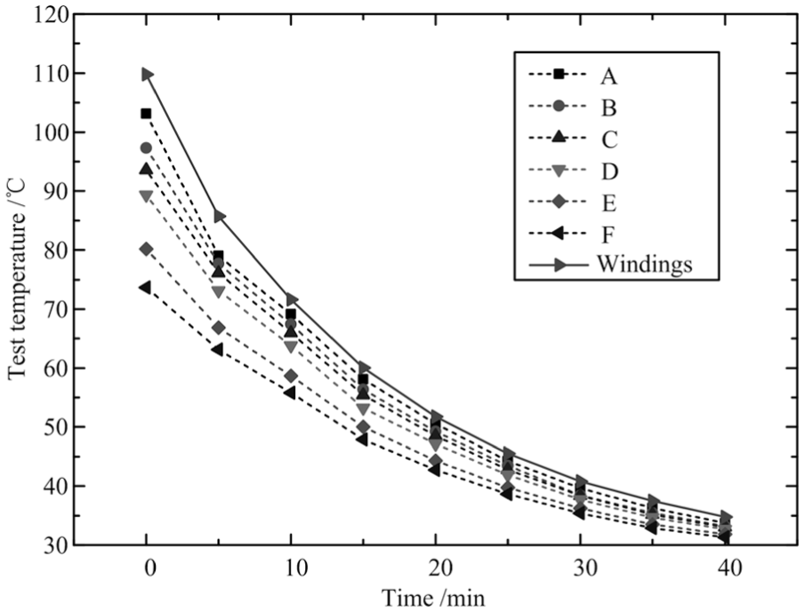
Cooling curves of the ELA’s inside coils and outside temperature test points.

From Figure 12, after the ELA stops working, temperature test points and moving coils cool down in approximate exponential relationship under the natural air cooling condition. The temperature differences among all test points are rapidly disappearing, and it finally reaches to a stable normal state. The average temperature of the coils is much higher than that of outside temperature test points but close to the average value of temperature rise inside the coils through simulation calculation.

Now, it compares simulation calculation data with temperature test data so as to check and verify the accuracy and reliability of the previous temperature field simulation model. Figure 13 shows comparison between the ELA’s simulation and temperature rise test with engine speed of 3000 r/min, and Figure 13(b) does single out the contrast relation between simulation and test data in two temperature maximum–minimum points: points A and F. The results show that the simulation is coincidence with the test data while the highest error between them is 6.54% within the error allowed. Finally, it strongly verifies the accuracy of the temperature and electromagnetic fields’ coupling simulation model.

Figure 13.

Comparison between the ELA’s simulation and temperature rise test with engine speed of 3000 r/min.

Research on the temperature rise law of the ELA

Through methods of both simulation and test, the temperature distribution and temperature rise changing relationship are obtained. Next, it will further analyze the temperature rise law of the ELA.

It can be found from Figure 7 that the temperatures of all points in the ELA increase with time and gradually reach a relatively steady state after 30 min. The relation of the outside points’ temperature value is A > B > C > D > E > F while that of the inside points’ temperature is W > X > Y > Z. The overall temperature tends to be lower from top to bottom in the axial direction. The main reason is the open of ELA’s bottom, so that it is convenient for heat convection with outer air. Additionally, the moving coils’ reciprocating motion inside the ELA is more favorable to heat convection. On the basis of temperature rise relation W > X > A, high heat source of the ELA mainly focuses on the winding coils. And because of different heat dissipation, the temperature of coils closer to the actuator’s heart is much higher.

Besides, the actuator’s temperature distribution is clear from the cloud chart of the ELA’s temperature in Figure 8. From this chart, the ELA’s high temperature points in the winding coils state that copper loss of the winding coils is the primary part of loss source during the actuator operation. The temperature distribution trends downward from top to down that is consistent with the analyzed results of the ELA’s heat transfer model in the previous section. In addition, distribution of the actuator’s internal temperature rise changes continuously when the actuator runs less than 30 min, but it becomes stable after 30 min until 70 min. This means the ELA nearly reaching a state of heat balance at 30 min which is in consistent with the temperature rise curve of all testing points analyzed earlier in this article.

The ELA’s temperature rises differently in different working conditions, but there exists certain laws. To explore the relation between the ELA’s temperature rise and working condition, temperature rise will be simulation calculated at four engine speeds such as 1500, 3000, 4500, and 6000 r/min, and thus, the change in the testing points’ temperature rise could be obtained as shown in Figure 14.

Figure 14.

Temperature rise change curves of the ELA’s temperature testing points at four working conditions.

As seen in Figure 14, the changes in the ELA’s temperature rise are similar under different working conditions. In the beginning, temperature of every testing points increases sharply with time, and it slows down and finally tends to be heat balance when reaching a critical time. Along with the engine speeding up, the critical time goes backward, and the stable temperature value is higher reaching the heat balance condition. Hence, the changes in the ELA’s temperature rise can be divided into three areas as shown in Figure 11(a): rapidly rising area, slowly rising area, and heat balance stable area. All cases of the actuator’s temperature rise under different working conditions accord with this law. However, there are differences in starting time and maintain time of each area.

Furthermore, it can be found through the aspect of all temperature testing points’ differences that when the ELA reaches a stable state of heat balance, temperature differences between the highest point A and lowest point F of the outer testing points show an increasing trend with faster engine speed. This mainly relates to cooling condition of the heat source position and different temperature testing points.

For the purpose of further analysis on the comparison of the ELA’s temperature rise under different working conditions, here it analyzes the temperature changes of two special positions: point A and point F in Figure 15. This figure illustrates that the ELA’s temperature increases more rapidly and needs longer time to reach a heat balance stable condition when the engine revolves up faster. Although the temperature of all testing points grows sharply, it will decline with increasing engine speed that is mainly because of cooling and dissipating heat in a large space. In other words, cooling capacity of the outside air and inner motion of the ELA cause heat convection which leads to suppression in the ELA’s temperature rise in high-speed operation.

Figure 15.

Temperature rise change curves of monitoring points A and F under different working conditions.

Conclusion

From the perspective of thermodynamics, this article analyzes the thermogenesis of the ELA applied in the EDVT and also studies the heat transfer process of the ELA in depth based on the heat transfer theory. Through analysis, some regular conclusions are as follows:

1. With changing times, temperature generated in the normal operation of the ELA can be divided into three areas: rapidly rising area, slowly rising area, and heat balance stable area. All cases of the actuator’s temperature rise under different working conditions accord with this law.

2. The overall temperature of the ELA tends to be lower from top to bottom in the axial direction. In addition, based on the temperature rise relation W > X > A, high heat source of the ELA mainly focuses on the winding coils. And because of different heat dissipations, the temperature of coils closer to the actuator’s heart is much higher.

3. By comparison of the ELA’s temperature rise at different working conditions, results show that when the engine speed is faster, the ELA’s temperature increases more rapidly and needs longer time to reach a heat balance stable condition.

The conclusions obtained in this article are original and reflect the temperature distribution and variation of the ELA. The results of the study will provide important technical support for the follow-up research of the actuator’s cooling technology and indicate the analysis direction of cooling scheme.