The economic benefit of liner ships with lower speed

Abstract

In recent years, the proportion of fuel costs in the total shipping costs grows up with the increase in international crude oil price. The rising cost seriously restricts the development of shipping enterprises. Many researches and cases show that reducing the ship’s fuel consumption by cautiously and reasonably decelerating the ship is the most simple and effective mean to control the shipping cost. However, the transportation time is longer when the speed is reduced. In other words, shipper would have to pay more for per unit transportation time. When the increase in transit time exceeds a certain range, liner companies are likely to lose customers. This article aims to maximize the profit of a liner company, which consisted of the variety of fuel cost, fixed cost, operating cost, and other related factors. And at the same time, the change in the shipper’s transport time cost and freight cost is considered. Then, a speed–freight optimization model based on the bat algorithm is established using MATLAB toolbox, in which the liner line is segmented. Finally, this article uses the model to optimize the route of the Far East to North America. The results show that the model can guarantee the quality of transport and reduce transport cost by adjusting speed at the same time.

Introduction

Requirement of shipping is derived from the demand of international trade; liner ship has the task of undertaking Chinese international trade transportation. In addition to tremendous initial building and purchasing cost, liner ships have to pay huge fuel oil expenses in the sequence of voyages in everyday operation. Compared with other costs (such as maintenance cost, tax, and insurance), fuel oil cost takes an important part in shipping cost, reaching 40% and seeming to be total of other tax. ¹ Under such severe condition, a number of owners of the vessel take action of lowering speed; as a result, they acquire obvious effects. How to set the speed of vessel in operation, supply superior service for clients, and decrease operation cost have already become one of the important decisions in liner ship. In addition, to achieve sustainable development in Chinese economic, China comes up with energy conservation and emission reduction in transportation. Ships consume lots of energy; fuel consumption takes up 30% in world consumption. On one hand, high fuel consumption brings tremendous pollution. On the other hand, it also brings high operation cost. So, how to reduce the pollution of the transportation industry becomes the most important component of Chinese energy conservation and emission reduction strategy. Lower speed of ship saves a large number of fuel oil cost for liner ship. However, to the owner of cargo, time of transportation prolongs yet. If liner ships only pay close attention to its own cost and ignore the profit of the owner of cargo, they may lose valuable client resource. Therefore, lowering speed and energy conservation, reducing waste resource, and maximizing the profit of the owner of cargo and liner ship have become an important study issue.

At present, most studies on optimization of liner shipping services have assumed that ships sail at a given speed.^2–9 With the study and development of new type engine and fuel, ships can use one or more types of fuels. ¹⁰ And because new types of engines have higher hot ratio than diesel engine, ships mainly adopt diesel engine currently. Hu et al. ¹¹ considered that sailing in constant speed was an important regular pattern for the energy conservation of shipping. Kakoi et al. ¹² systematically analyzed lower speed in economic and the influence when it changes. Christiansen et al. ² analyzed that the nonlinearity effects brought by changes in ship’s speed led to changes in planning decision of fleet and deduced mathematic relation among ship’s speed, ship arrive and depart time, cost of the sequence of voyages or flights, and number of ships in ship route and established mixed integer nonlinearity fleet programming model. Wang and Meng ⁶ investigated the optimal sailing speed of container ships on each leg of each ship route in a liner shipping network while considering transshipment and container routing and proposed an efficient outer-approximation method to an optimal solution with a predetermined optimality tolerance level. Wang and Meng ⁷ first calibrated the bunker consumption—sailing speed relation for container ships using historical operating data from a global liner shipping company. Chang et al. ¹³ proposed an ant colony optimization algorithm to solve the traffic counting location problem by explicitly generating the Pareto solutions. By introducing additional suitable intensification mechanisms, the nondominated solutions can be attained with significantly fewer iterations and ants, which consequently indicate the effectiveness of the system and further verifies the modeling capability of ant colony optimization. Korsvik et al. ¹⁴ used the control variable method to study the effects of fluctuations of fuel prices and variation of the fixed costs on the average daily earning of each voyage, and the optimization model of tramp vessel speed was constructed with the object of average daily earnings maximization. Norstad et al. ¹⁵ presented the tramp ship routing and scheduling problem with speed optimization, where speed on each sailing leg was introduced as a decision variable, and they presented a multi-start local search heuristic to solve this problem.

On the basis of finishing sailing, we come up with a model about optimizing liner ship speed, which can save the cost as well as guarantee the quality of transportation. This article’s main work is in several aspects as follows:

1. Analyzing the reason and superior of lower speed.

2. Analyzing the relationship between speed and Bunker adjustment factor (BAF), the relationship between speed and number of ships, and the relationship between speed and operation cost, so that we can measure the liner operators’ profit.

3. Analyzing the time value of owner of cargo, we reach the acceptable boundary to owner of cargo bonding cost.

4. Combining with above-mentioned analysis, we set up optimized speed model of liner ship, solving by bat algorithm (BA) and proceeding instance analysis with the United States and China the container liner routes.

There are two main contributions in this article. On one hand, we consider that the speed is different in the different segments, which is different from most speed optimization problems with single speed in the whole shipping routes. On the other hand, heuristic algorithm is a feasible way of solving problems in practical problems, and BA is one of the new heuristic algorithms. At present, BA is mainly applied in vehicle routing problem, scheduling problem, and so on. We explored the application of BA in the field of maritime transport for the parameter optimization in the maritime problems.

The objectives of this study are to achieve the maximum profit in condition of lowering speed. Thus, this article is structured as follows: section “Speed–cost optimization model” provides brief introduction on speed–cost optimization model which includes problem description, model assuming, and speed–cost optimization model; section “BAs” provides the introduction of BA and the method to solve the model; section “Case studies” provides the case study to check the effect in condition of lowering speed; and section “Conclusion” provides the conclusion.

Speed–cost optimization model

Problem description

The object that we choose to study is the fleet under the condition of high fuel oil cost. According to the information and forecast of transportation needs in the future, we lower the speed to make the liner voyage profit maximization. However, the market competition may be influenced when reducing speed cautiously and reasonably. ¹⁶ Thus, we adjust ratio of freight and add ships to current lines at the same time, so that we can guarantee the level of service and reserve clients, as shown in Figure 1.

Figure 1.

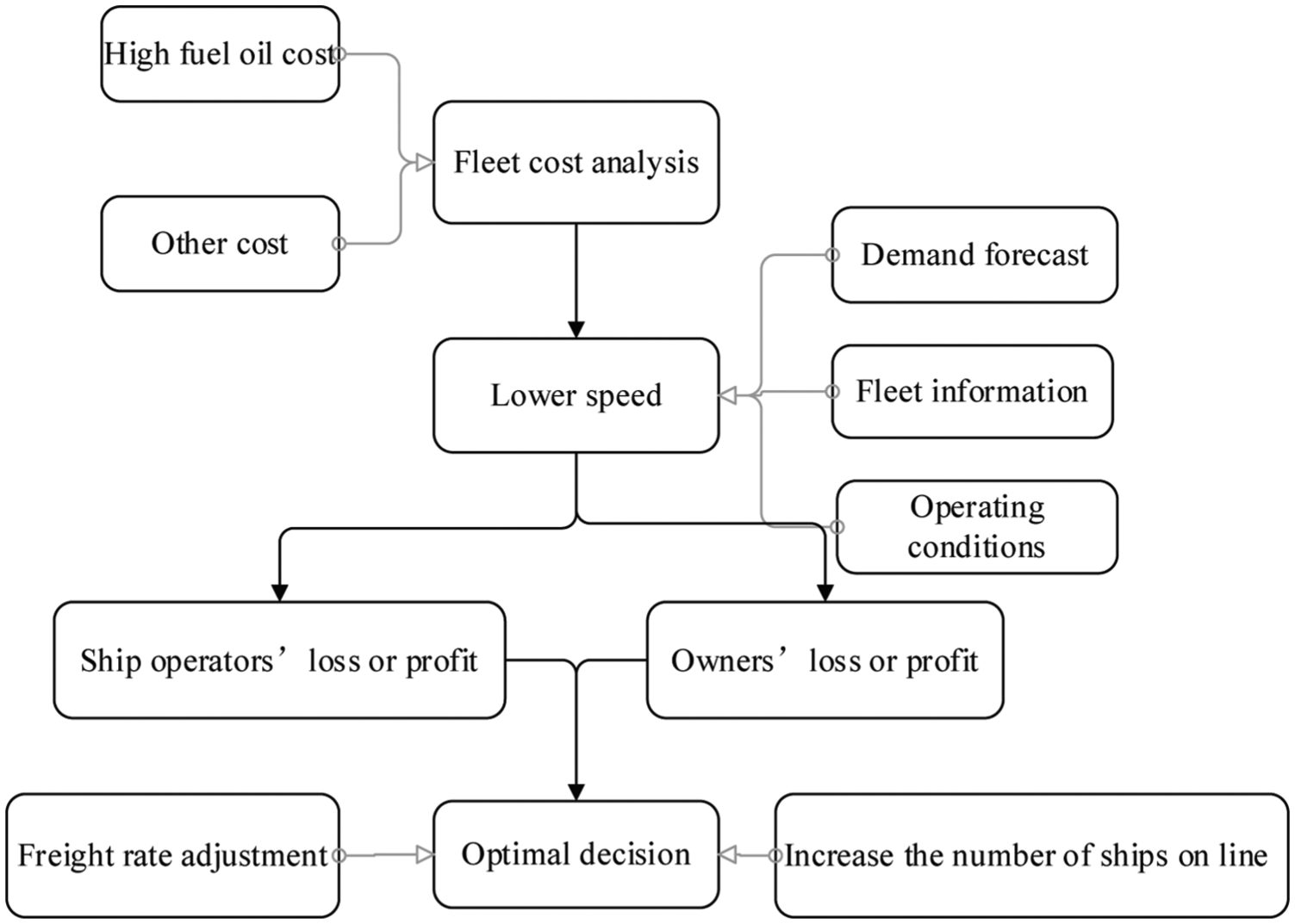
The level of service and reserve clients.

In Figure 1, first we analyze the component of fleet cost that contains the high fuel oil cost and other cost (e.g. fixed cost and variable cost). Then, the lower speed can be determined by some factors such as demand forecast, fleet information, and operating condition. So, we can figure out the loss or profit of the ship operators’ and owners’, respectively. Finally, the optimal decision about freight adjustment or increase the number of ships on line can be provided for the decision makers.

This article establishes math model to make the best decision against problem as follows:

1. Number of ships in shipping routes;

2. Either purchasing new liner or not;

3. The optimal speed of liner in each segment;

4. Either adjust the freight ratio in each segment or not and the adjustment extent.

Model assuming

To make the model approach the fact of liner operation, we set several hypothesizes before setting up model:

1. 1 Type of ship is the same, age of ship is near, and the effect of different ages on shipping cost can be ignored in the whole shipping routes;

2. Study period is in years, starting at first year and terminating at year t. Behavior of buying occurs at the beginning of a year and expenses of operation cost occurs at the end of this year. Funds are discounted at the beginning of this year, and the discount ratio is e;

3. Ships bought before study period is ships which have been purchased, and decisions have no influence on these ships in the study period. Cost of buying these ships is ignored in the model;

4. Liner companies keep the schedule frequency to retain clients after lowering the speed;

5. Time of loading, unloading, and waiting is invariable in each port after lowering the speed;

6. Shipping routes is long, and natural condition is different in different segments. Some natural condition may affect speed, such as flow speed. Thus, we divide the shipping routes into n segments;

7. Freight ratio is related to the kind of cargo; thus, we divide the cargo into K types;

8. When the ship’s speed changes, various factors change at the same time, so this article mainly catches the changes in fuel oil cost, operating cost, and number of ships and analyzes profit and loss;

9. In terms of shipper, lower speed can prolong transport time, and in terms of liner shipping, most of the shippers are not sensitive to transport time. But if the speed was too low, shipper might choose other liner companies, so we assume that the lowest is 13 knot in this article;

10. After lowering the speed, liner companies adjust freight ratio to retain clients. We assume that the ratio of shippers’ transport cost is no more than 10% in every segment;

11. When lowering the speed, we adjust the ratio of freight and add ships to current lines. Thus, assuming that the market of liner shipping company is unchanged and is reasonable.

Speed–cost optimization model

Decision variables are $\mathrm{V}{\prime }_{\mathrm{i}}$ and $\mathrm{f}{\prime }_{\mathrm{ij}}$ , which is the speed after lowering, and the objective function is shown in equation (1)

$$\begin{array}{l}\mathrm{maxNPV}=\mathrm{g}\left(\mathrm{V}{\prime }_{\mathrm{i}},\mathrm{f}{\prime }_{\mathrm{ij}}\right)=\frac{{\left(1+\mathrm{e}\right)}^{\mathrm{t}}-1}{\mathrm{e}\times {\left(1+\mathrm{e}\right)}^{\mathrm{t}}}\\ \times \left(\mathrm{\Delta }{\mathrm{R}}^{\mathrm{f}}-\mathrm{\Delta }{\mathrm{C}}^{\mathrm{F}}-\mathrm{\Delta }{\mathrm{C}}^0\right)\times \mathrm{m}\prime -\mathrm{\Delta }\mathrm{m}\times {\mathrm{C}}^{\mathrm{S}}\\ \mathrm{j}=1,2,\mathrm{\dots },\mathrm{K};\mathrm{i}=1,2,\mathrm{\dots },\mathrm{N};\mathrm{t}=0,1,\mathrm{\dots }\end{array}$$

(1)

Solving of $\mathrm{\Delta }{\mathrm{C}}^{\mathrm{F}}$ , $\mathrm{\Delta }{\mathrm{C}}^0$ , and $\mathrm{\Delta }\mathrm{m}$ can be made using the following equation

$$\begin{array}{l}\mathrm{\Delta }{\mathrm{C}}^{\mathrm{F}}={\mathrm{C}}^{\mathrm{F}\prime }-{\mathrm{C}}^{\mathrm{F}}={\mathrm{P}}^{\mathrm{FH}}\times \delta \times {\displaystyle \sum _{\mathrm{i}=1}^{\mathrm{N}}\left({\mathrm{V}}_{\mathrm{i}}^{2\prime }-{\mathrm{V}}_{\mathrm{i}}^2\right)\times \frac{\mathrm{n}\times {\mathrm{L}}_{\mathrm{i}}}{24}}\\ +{\mathrm{G}}^{\mathrm{FL}}\times {\mathrm{P}}^{\mathrm{FL}}\times {\displaystyle \sum _{\mathrm{i}=1}^{\mathrm{N}}\frac{\mathrm{n}\times {\mathrm{L}}_{\mathrm{i}}}{24}\left(\frac{1}{\mathrm{V}{\prime }_{\mathrm{i}}}-\frac{1}{{\mathrm{V}}_{\mathrm{i}}}\right)}\end{array}$$

(2)

where $\mathrm{\Delta }{\mathrm{C}}^{\mathrm{F}}$ is the annual save of fuel oil consumption cost (dollar), $\mathrm{V}{\prime }_{\mathrm{i}}$ is the speed after changing in the i segment (knot), ${\mathrm{P}}^{\mathrm{FH}}$ is the price of heavy oil (dollar/t), ${\mathrm{P}}^{\mathrm{FL}}$ is the price of light oil (dollar/t), ${\mathrm{L}}_i$ is the route distance of liner ship in the i segment (n mile), $\mathrm{n}$ is the annual voyage number of ships (times/year), $\delta$ is the coefficient of fuel oil consumption, ${\mathrm{G}}^{\mathrm{FL}}$ is the light oil daily consumption (t/day), and ${\mathrm{C}}^{\mathrm{S}}$ is the additional cost after adding another ship (dollar/ship).

The operating cost increases as the voyage time increases

$$\mathrm{\Delta }{\mathrm{C}}^0={\mathrm{C}}^{0\prime }-{\mathrm{C}}^0=\mathrm{A}\times \sum _{\mathrm{i}=1}^{\mathrm{N}}\frac{\mathrm{n}\times {\mathrm{L}}_{\mathrm{i}}}{24}(\frac{1}{{\mathrm{V}}_{\mathrm{i}}\prime }-\frac{1}{{\mathrm{V}}_{\mathrm{i}}})$$

(3)

where $\mathrm{\Delta }{\mathrm{C}}^0$ is the increased operating cost under lower speed (dollar), ${\mathrm{C}}^{0\prime }$ is the operating cost under lower speed (dollar), ${\mathrm{C}}^0$ is the operating cost before lower speed (dollar), and $\mathrm{A}$ is the daily operating cost (dollar/day).

When the speed of ships decreases from ${\mathrm{V}}_{\mathrm{i}}$ to ${\mathrm{V}}_{\mathrm{i}}\prime$ , the number of ships increases

$$\mathrm{\Delta }\mathrm{m}=\mathrm{m}\prime -\mathrm{m}=\frac{{\mathrm{n}}^2}{{\mathrm{T}}^{\mathrm{c}}}\sum _{\mathrm{i}=1}^{\mathrm{N}}\frac{{\mathrm{L}}_{\mathrm{i}}}{24}(\frac{1}{{\mathrm{V}\prime }_{\mathrm{i}}}-\frac{1}{{\mathrm{V}}_{\mathrm{i}}})$$

(4)

where $\mathrm{m}\prime$ is the ship numbers of the whole shipping routes, $\mathrm{\Delta }\mathrm{m}$ is the changed numbers of ship after lowering the speed, and ${\mathrm{T}}^{\mathrm{c}}$ is the annual operation time of ships.

Transportation revenue reduces with the reducing turnover rate after lowering the speed

$$\mathrm{\Delta }{\mathrm{R}}^{\mathrm{f}}={\mathrm{R}}^{\mathrm{f}\prime }-{\mathrm{R}}^{\mathrm{f}}$$

(5)

where $\mathrm{\Delta }{\mathrm{R}}^{\mathrm{f}}$ is the increased transportation revenue after lowering the speed (dollar), ${\mathrm{R}}^{\mathrm{f}\prime }$ is the transportation revenue after lowering the speed (dollar), and ${\mathrm{R}}^{\mathrm{f}}$ is the transportation revenue before lowering the speed (dollar).

Constraint

$$\begin{array}{l}{\displaystyle \sum _{\mathrm{i}=1}^{\mathrm{N}}{\displaystyle \sum _{\mathrm{j}=1}^{\mathrm{K}}{\mathrm{Q}}_{\mathrm{i},\mathrm{j}}}}\times {\mathrm{f}}_{\mathrm{ij}}\prime \ge \left\{\left(\frac{\mathrm{n}\times {\mathrm{L}}_{\mathrm{i}}}{24{\mathrm{V}\prime }_{\mathrm{i}}}+{\mathrm{T}}_{\mathrm{i}}^{\mathrm{UL}}+{\mathrm{T}}_{\mathrm{i}}^{\mathrm{L}}+{\mathrm{T}}_{\mathrm{i}}^{\mathrm{W}}\right)\times \mathrm{A}\right\}+{\displaystyle \sum _{\mathrm{i}=1}^{\mathrm{N}}{\mathrm{C}}_{\mathrm{i}}^{\mathrm{ETC}}}\\ +\left\{{\mathrm{P}}^{\mathrm{FH}}\times \delta {\displaystyle \sum _{\mathrm{i}=1}^{\mathrm{N}}\frac{\mathrm{n}\times {\mathrm{L}}_{\mathrm{i}}}{24{\mathrm{V}\prime }_{\mathrm{i}}}}\times \mathrm{V}{\prime }_{\mathrm{i}}^3+{\mathrm{P}}^{\mathrm{FL}}\times {\mathrm{G}}^{\mathrm{FL}}{\displaystyle \sum _{\mathrm{i}=1}^{\mathrm{N}}\left(\frac{\mathrm{n}\times {\mathrm{L}}_{\mathrm{i}}}{24{\mathrm{V}\prime }_{\mathrm{i}}}+{\mathrm{T}}_{\mathrm{i}}^{\mathrm{UL}}+{\mathrm{T}}_{\mathrm{i}}^{\mathrm{L}}+{\mathrm{T}}_{\mathrm{i}}^{\mathrm{W}}\right)}\right\}\end{array}$$

(6)

$$\sum _{\mathrm{j}=1}^{\mathrm{K}}{\mathrm{Q}}_{\mathrm{ij}}\le \mathrm{DWT}-\sum _{\mathrm{i}=1}^{\mathrm{i}-1}\sum _{\mathrm{j}=1}^{\mathrm{K}}{\mathrm{Q}}_{\mathrm{i}-1,\mathrm{j}}+\sum _{\mathrm{i}=1}^{\mathrm{i}}\sum _{\mathrm{j}=1}^{\mathrm{K}}\mathrm{UL}{\mathrm{Q}}_{\mathrm{i}-1,\mathrm{j}}$$

(7)

$$\mathrm{0}\le {\mathrm{e}}_{\mathrm{z},\mathrm{z}+\mathrm{d},\mathrm{j}}={\displaystyle \sum _{\mathrm{i}=\mathrm{z}}^{\mathrm{z}+\mathrm{d}}\frac{{\mathrm{C}}_{\mathrm{i}}^{\mathrm{T}}+{\mathrm{F}}_{\mathrm{ij}}}{{\mathrm{C}}_{\mathrm{i}}^{\mathrm{T}\prime }+\mathrm{F}{\prime }_{\mathrm{ij}}}}\le 10\%$$

(8)

$$13\le {\mathrm{V}\prime }_{\mathrm{i}}\le {\mathrm{V}}_{\mathrm{i}}\le {\mathrm{V}}_{\max }$$

(9)

$$\sum _{\mathrm{i}=1}^{\mathrm{N}}{\mathrm{T}\prime }_{\mathrm{i}}\times \mathrm{n}-{\mathrm{T}}^{\mathrm{C}}\times \mathrm{m}\prime =0$$

(10)

where ${\mathrm{f}}_{\mathrm{ij}}$ is the freight rates of liner shipping for the j cargo in the i segment, ${\mathrm{T}}_{\mathrm{i}}^{\mathrm{UL}}$ is the annual unloading time in port of loading in the i segment (days), ${\mathrm{T}}_{\mathrm{i}}^{\mathrm{L}}$ is the annual loading time in port of unloading in the i segment (days), ${\mathrm{T}}_{\mathrm{i}}^{\mathrm{W}}$ is the annual berth time in the i segment except loading and unloading time (days), dead weight tonnage ( $\mathrm{DWT}$ ) is the maximum dead weight ton of ship (ton), ${\mathrm{ULQ}}_{\mathrm{i},\mathrm{j}}$ is the unloading amount of the j cargo in the i segment (ton), and ${\mathrm{V}}_{\max }$ is the designed speed of ships (n mile).

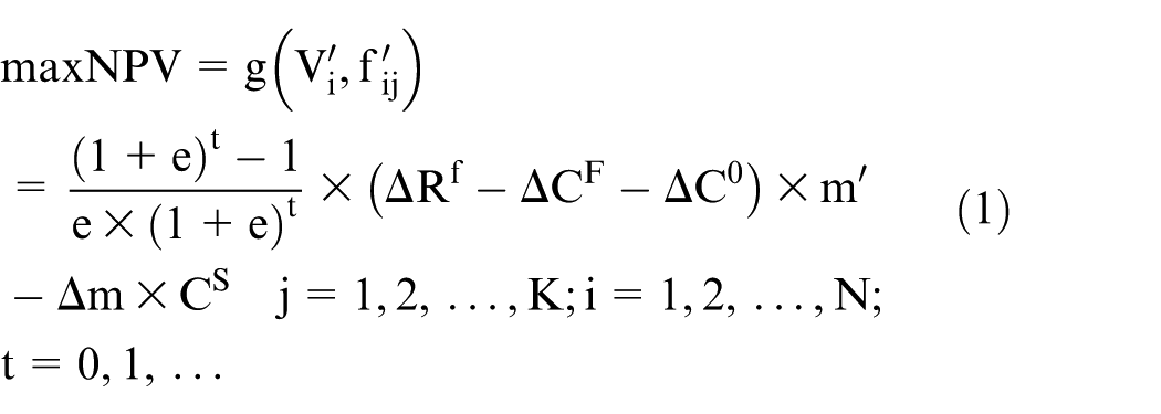
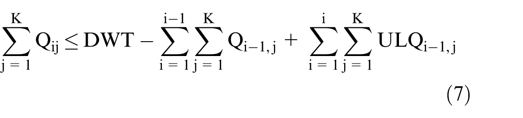
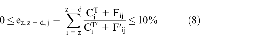
Equation (1) is the objective function of liner companies, and in the condition of high price of fuel oil, liner companies adjust speed and increase the number of ships in shipping routes, to acquire the highest net present value (NPV) in condition of guaranteeing the rate of voyage. The residual ones are constraints: equation (6) is constraint of cost, requiring that every ship’s income must be higher than cost; equation (7) is constraint of load, requiring that weight of cargo which is loaded in port must be less than the difference of total DWT and existing cargo’s DWT; equation (8) is constraint of rate of transport cost, requiring that the sum ratio of transport time cost and freight cost is no more than 10%; equation (9) is constraint of speed, requiring that speed should be higher than 13 knot and less than maximum speed after lowering the speed; and equation (10) is the constraint of frequency of voyage, requiring that liner companies keep the frequency by increasing the number of ships after lowering the speed.

BAs

The above model is a nonlinear programming problem, which contains two continuous variables, and objective function and constraints are nonlinear; against these feature of this model, this article improves the BAs, solving the model with MATLAB.

Many literatures suggested that heuristic algorithms were good choice to solve this kind of problems.^17–20 The BA is a heuristic algorithm proposed by Yang ²¹ and Cheng, ²² which has been widely used in the literature.^23,24 The algorithm is a kind of effective method to search the global optimal solution based on iterative optimization technique. First, it was initialized to a group of random solutions and then through the iterative search for the optimal solution. Next, the optimal solution improves the local search by random flight around local data processing. Compared with other algorithms, BA is far superior to other algorithms in terms of accuracy and effectiveness and not many parameters to adjust.

This heuristic algorithm is inspired by the echolocation behavior. Bats emit a very loud sound pulse and listen for the echo that returns from objects. Bats fly randomly with frequency, velocity, and position when searching for prey. The BA is formulated to imitate the process of bats to find their prey. In BA, each bat represents a solution in the population. The frequency, velocity, and position of each bat are changed for further movement. The changing frequency provides the diversity of the solutions. For using the variation of frequency, BA can be considered as a frequency tuning algorithm to provide a balanced combination of exploration and exploitation during the search process. The BA considers many simplification and idealization rules of bat behaviors by Yang ²¹ and Cheng. ²² The algorithm involves a series of iterations. A set of solutions changes in these iterations. If the new solution is accepted, the loudness and pulse rate are changed. The frequency, velocity, and position of the solutions are formulated as in equations (11)–(13)

$${\mathrm{f}}_{\mathrm{i}}={\mathrm{f}}_{min}+({\mathrm{f}}_{max}-{\mathrm{f}}_{min})\mathrm{\beta }$$

(11)

$${\mathrm{v}}_{\mathrm{i}}^{\mathrm{t}}={\mathrm{v}}_{\mathrm{i}}^{\mathrm{t}-1}+({\mathrm{x}}_{\mathrm{i}}^{\mathrm{t}-1}-{\mathrm{x}}_{\mathrm{gbest}}^{\mathrm{t}}){\mathrm{f}}_{\mathrm{i}}$$

(12)

$${\mathrm{x}}_{\mathrm{i}}^{\mathrm{t}}={\mathrm{x}}_{\mathrm{i}}^{\mathrm{t}-1}+{\mathrm{v}}_{\mathrm{i}}^{\mathrm{t}}$$

(13)

where $\beta$ is a random number between [0, 1]; ${\mathrm{f}}_{\mathrm{i}}$ is the frequency of the $\mathrm{ith}$ bat in a range $[{\mathrm{f}}_{min},{\mathrm{f}}_{max}]$ to avoid unacceptable increase in velocity, and in such case, the position may land up in some imaginary search space; ${\mathrm{v}}_{\mathrm{i}}$ and ${\mathrm{x}}_{\mathrm{i}}$ correspond to the velocity and position of $\mathrm{ith}$ bat, respectively; and ${\mathrm{x}}_{\mathrm{gbest}}^{\mathrm{i}}$ represents the global best at step $\mathrm{t}$ . For the local search, once a solution is selected among the current best solutions, this local search generated a new solution for each bat using random walk as shown in equation (14)

$${\mathrm{x}}_{\mathrm{new}}={\mathrm{x}}_{\mathrm{old}}+\epsilon {\mathrm{A}}^{\mathrm{t}}$$

(14)

The value of $\epsilon$ is a random number between [−1,1] and ${\mathrm{A}}^{\mathrm{t}}$ is the average loudness of all the bats at step $\mathrm{t}$ .

The loudness decreases and the pulse rate increases when a bat finds its prey. It means that the loudness and the pulse are changed in each iteration. The loudness and the pulse are changed based on the following equations

$${\mathrm{A}}_{\mathrm{i}}^{\mathrm{t}+1}=\mathrm{\alpha }{\mathrm{A}}_{\mathrm{i}}^{\mathrm{t}}$$

(15)

$${\mathrm{r}}_{\mathrm{i}}^{\mathrm{t}+1}={\mathrm{r}}_{\mathrm{i}}^0[1-\exp (-\mathrm{\gamma }\mathrm{t})]$$

(16)

where $\alpha$ is a constant value in the range of $[0,1]$ and $\gamma >0$

Variable coding

The decision variables are $\mathrm{V}{\prime }_{\mathrm{i}}$ and $\mathrm{f}{\prime }_{\mathrm{ij}}$ , whose range is $\mathrm{V}{\prime }_{\mathrm{i}}\in [{\mathrm{V}}_{\min },{\mathrm{V}}_{\max }]$ and $\mathrm{f}{\prime }_{\mathrm{ij}}\in [{\mathrm{f}}_{\min },{\mathrm{f}}_{\max }]$ , respectively; binary encoding with lengths ${\mathrm{k}}_{\mathrm{v}}$ and ${\mathrm{k}}_{\mathrm{f}}$ and producing 2k coding, the accuracy is shown in equation (17)

$${\partial }_{\mathrm{v}}=\frac{{\mathrm{V}}_{\max }-{\mathrm{V}}_{\min }}{2^{{\mathrm{k}}_{\mathrm{v}}}-1},{\partial }_{\mathrm{f}}=\frac{{\mathrm{f}}_{\max }-{\mathrm{f}}_{\min }}{2^{{\mathrm{k}}_{\mathrm{f}}}-1}$$

(17)

The problem is multivariable; two variables are encoded, and lengths are ${\mathrm{k}}_{\mathrm{v}}$ and ${\mathrm{k}}_{\mathrm{f}}$ . Then, the two are linked into a long string encoding, $\mathrm{k}={\mathrm{k}}_{\mathrm{v}}+{\mathrm{k}}_{\mathrm{f}}$ ,which is coding of problem, respectively, and can be decoded when decoding.

Population initialization

Initial population is the starting point of BAs. To guarantee the feasibility and diversity of individual in group, randomly generated initial individuals based on constraints has been used to make the initial population generate feasibly.^25,26

Fitness function

In standard BA, the value of fitness function is nonnegative, and it requires that the optimization problem is transformed into a maximization problem. The objective function is the sake of great value in the form of conversion in application time and mapping nonnegative fitness function. We chose objective $(max\mathrm{NPV}=\mathrm{g}(\mathrm{V}{\prime }_{\mathrm{i}},\mathrm{f}{\prime }_{\mathrm{ij}}))$ as fitness function. ²⁷

The pseudo code of the BA

To run the BA, the main steps are as follows (Figure 2):

• Step 1. Initialize the bat population or their position ${\mathrm{x}}_{\mathrm{i}}$ and their velocities ${\mathrm{v}}_{\mathrm{i}}$ . Define pulse frequency ${\mathrm{f}}_{\mathrm{i}}$ at ${\mathrm{x}}_{\mathrm{i}}$ . Initialize the loudness ${\mathrm{A}}_{\mathrm{i}}$ and pulse rates ${\mathrm{r}}_{\mathrm{i}}$ ;

• Step 2. Generate new solutions by adjusting frequency and update velocities and positions using equations (11)–(13);

• Step 3. If (rand > r_i), select a solution among the best solutions. Generate a local solution around the selected best solution;

• Step 4. Else generate a new solution by flying randomly;

• Step 5. If $(\mathrm{rand}<{\mathrm{A}}_{\mathrm{i}}\&\&\mathrm{f}({\mathrm{x}}_{\mathrm{i}})<\mathrm{f}({\mathrm{x}}_{\mathrm{best}}))$ , where $\mathrm{f}(.)=\mathrm{objective\; function\; min}\mathrm{NPV}$ , accept the new solutions, increase ${\mathrm{r}}_{\mathrm{i}}$ , and reduce ${\mathrm{A}}_{\mathrm{i}}$ ;

• Step 6. Rank the bats and find the current best position;

• Step 7. While (iteration < maximum number of iterations n), the BA stops until the stop condition is met or meets the evolution algebra.

Figure 2.

The bat algorithm flowchart.

To run the BA, first is to initialize the bat population, which is their position ${\mathrm{x}}_{\mathrm{i}}$ and their velocities ${\mathrm{v}}_{\mathrm{i}}$ . Then, define pulse frequency ${\mathrm{f}}_{\mathrm{i}}$ at ${\mathrm{x}}_{\mathrm{i}}$ and initialize the loudness ${\mathrm{A}}_{\mathrm{i}}$ and pulse rates ${\mathrm{r}}_{\mathrm{i}}$ . Generate new solutions by adjusting frequency and update velocities and positions. Next, to see whether rand > A_i, if it is, select a solution among the best solutions and generate a local solution around the selected best solution. Else, generate a new solution by flying randomly. The next step, find whether rand < A_i && F(x_i) < F(x_best), if it is yes, accept the new solutions, increase ${\mathrm{r}}_{\mathrm{i}}$ , reduce ${\mathrm{A}}_{\mathrm{i}}$ , rank the bats, and find the current best position. Else, keep the current solution to the next step. Then, check whether iteration less than maximum number of iterations n, if not, go back to step 2. The BA stops until the stop condition is met or meets the evolution algebra.

Case studies

This article selects a traditional China–USA container route, Far East to US East, operating with nine ships which are 4250 TEU. The anchored order is Ningbo, Shanghai, Bhushan, Panama Canal, New York, Wilmington, SaiFenna, Panama Canal, and Bhushan. Shipping route is shown in Figure 3. We divide the shipping route into nine segments, as shown in Table 1.

Figure 3.

Shipping routes.

Table 1.

Partition of shipping route.

Port of departure	Port of arrival	Segment number
Ningbo	Shanghai	1
Shanghai	Bhushan	2
Bhushan	Panama	3
Panama	New York	4
New York	Wilmington	5
Wilmington	SaiFenna	6
SaiFenna	Panama	7
Panama	Bhushan	8
Bhushan	Ningbo	9

Schedule and turnaround time are shown in Tables 2 and 3, respectively. In Table 2, Eta represents the arrival time of each port, and Etd represents the departure time of each port. The date in Table 2 is matched with sailing time in Table 4. First, we find the shipping line distance of each port with sea chart; then we obtain the average speed in each segment from logbook; then we collect parameter of shipping line and ship in Clarkson; and, finally, we substitute the data into speed optimized model and achieve optimized speed and adjusted freight with BA and genetic algorithm (GA). As shown in Table 4, the optimized speed is lower than the actual speed, and the BA optimized speed is lower than GA optimized speed. The performance of BA is better than GA in speed optimized model.

Table 2.

Far East–North America line arrival time table of liner.

Port	Eta	Time	Etd	Time
Ningbo	Sat	0	Sat	0
Shanghai	Sun	1	Mon	2
Bhushan	Wed	4	Wed	4
Panama	Sun	22	Sun	22
New York	Fri	27	Sat	28
Wilmington	Mon	30	Mon	30
SaiFenna	Tue	31	Wed	32
Panama	Sun	36	Sun	36
Bhushan	Wed	60	Thu	61
Ningbo	Sat	63	Sat

Table 3.

Far East–North America schedules.

From	To
	New York	Wilmington	SaiFenna
Ningbo	27	30	31
Shanghai	25	28	29
Bhushan	23	26	27

Table 4.

Far East–North America line optimized speed–freight.

Segment number	Route length (mile)	Sailing time (days)	Average speed (knot)
			Actual speed	GA after	BA after	Tabu after
1	86.5	0.5	13.50	13.20	13.00	13.00
2	518.5	2	14.87	14.00	13.69	13.72
3	10345.6	18	23.95	20.75	20.39	20.39
4	2276.9	5	18.97	17.52	16.80	17.10
5	479.1	2	14.55	13.56	13.48	13.21
6	206.7	1	14.50	14.11	13.98	13.75
7	1747.4	4	18.20	16.45	15.97	15.97
8	10292.8	24	17.87	15.12	14.32	14.42
9	476.5	2	15.50	14.53	14.12	14.62

GA: genetic algorithm; BA: bat algorithm.

In this article, VC++.NET 2003 is used to achieve two algorithms, and operating environment is the Pentium IV 2.93-GHz processor and 3 GB for the Windows platform. A large number of experiments to determine the parameters are set as follows: $\mathrm{n}=300,\mathrm{A}=0.9,\mathrm{r}=0.5,{\mathrm{f}}_{\min }=0,\mathrm{and}{\mathrm{f}}_{\max }=2$ for BA; Tabu length $\mathrm{TSL}=10$ ; the number of neighborhood solution $\mathrm{m}=200$ ; iterations $\mathrm{n}=500$ for Tabu search algorithm; and crossover operation p_c = 0.6 and mutation operation p_m = 0.05 for GA. The results can be seen in Table 4.

From the optimized data, we can see that it can guarantee the quality of service and reduce the fuel oil cost at the same time, and the reduction of fuel oil cost is obvious (Table 5). From Table 5, it can reduce more than 20% cost in some segments (numbers 3, 4, and 8) optimized by BA. It can also be attained that the solutions by the improved BA are better than the GA solutions. And the solutions optimized by BA and Tabu algorithm are close. The solutions of BA are better than Tabu algorithm in segment numbers 2, 4, and 8. The optimized solutions of freight are shown in Figure 7. It is obvious that the freight is lower than before in some voyages, and the BA and Tabu optimized freights are lower than GA optimized freight, which can guarantee the quality of service better (Table 6).

Table 5.

The fuel oil cost of Far East–North America optimized line.

Segment number	Fuel oil cost (dollar)
	Before	GA after	BA after	Tabu after
1	4636	4421	4215	4215
2	21,472	21,213	20,980	21,010
3	311,100	250,240	231,654	231,004
4	85,400	70,312	68,464	69,521
5	23,180	21,064	21,050	21,050
6	14,030	13,671	13,006	13,003
7	73,200	68,021	65,800	65,310
8	317,200	240,122	221,445	223,450
9	25,620	23,169	22,354	22,108

GA: genetic algorithm; BA: bat algorithm.

Table 6.

The freight of Far East–North America optimized line.

Segment number	Freight (Yuan/TEU)
	Before	GA after	BA after	Tabu after
1	2150	2150	2150	2150
2	2590	2401	2350	2300
3	2450	2450	2450	2450
4	2350	2322	2300	2310
5	2400	2400	2400	2400
6	2440	2405	2400	2400
7	2000	2000	2000	2000
8	2160	2160	2160	2160
9	2130	2130	2130	2130

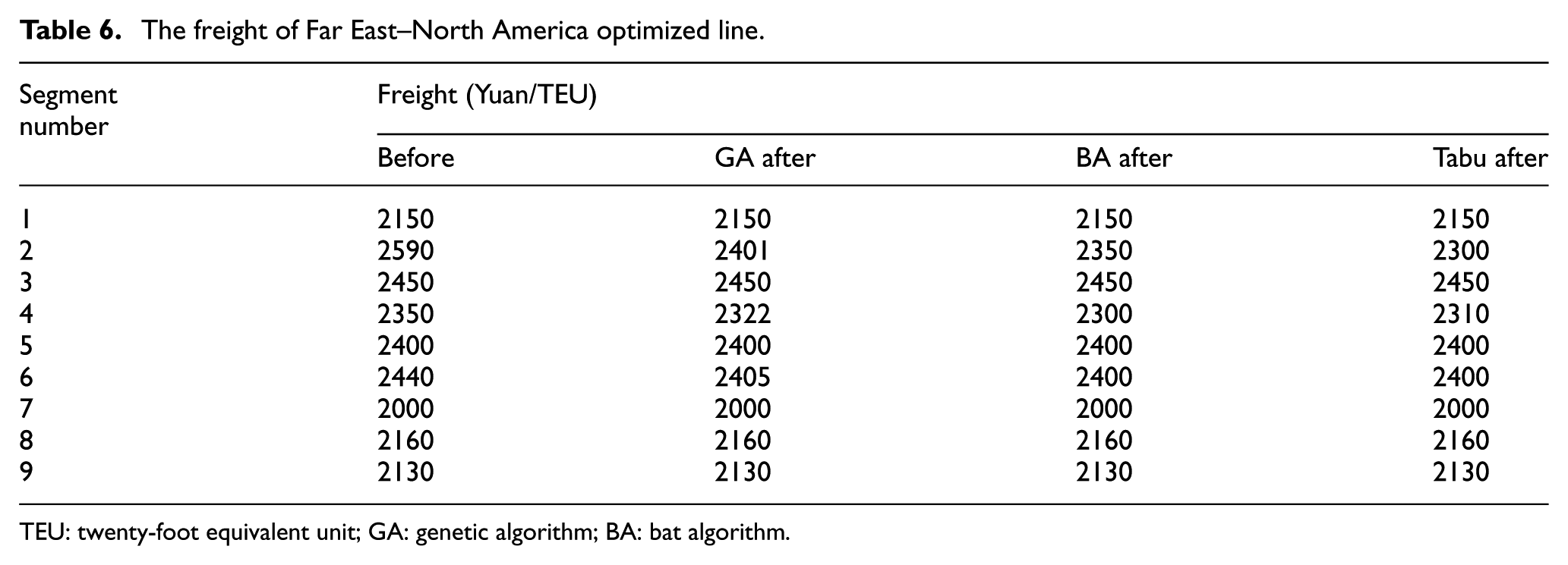
TEU: twenty-foot equivalent unit; GA: genetic algorithm; BA: bat algorithm.

To obtain the performance of the method in this article, the fuel oil cost and freight, which are achieved by BA, are shown in Figures 4 and 5, respectively. From Figure 4, we can see that the fuel oil cost of segments 3 and 8 is obviously decreased than before. In each segment, the solutions by the BA are smaller than actual fuel oil cost. From Figure 5, the freight of segment 2 is obviously decreased than before. The improved BA seems to be a powerful method for the speed–freight optimization model.

Figure 4.

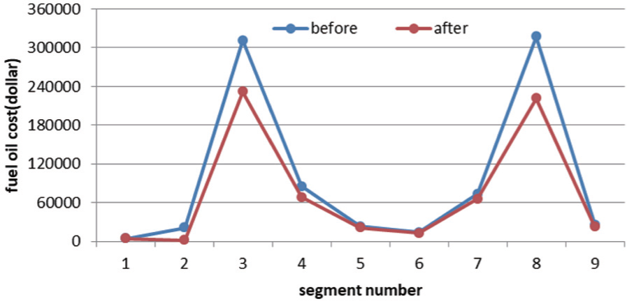
The fuel oil cost before and after optimization.

Figure 5.

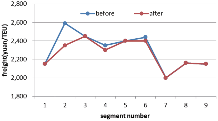
The freight before and after optimization.

To analyze the stability of the BA, we discuss the convergence of BA. Figure 6 shows its convergence of 10 experiments. We found that the target value of each experiment is almost stable eventually, and the optimal values of these 10 experiments are nearly the same, which are about 2,560,000 Yuan. Also, we can see that to obtain the best solution, BA used only 30 iterations, which is very effective. Thus, solving the problem by BA is reasonable and powerful. Furthermore, we compared BA, GA, and Tabu in Figure 7. There are 10 experiments for each algorithm. As can be seen from Figure 7, the volatility of Tabu is slightly larger, but the best solution of all experiments is found by the optimization of Tabu. And the volatilities of BA and GA are smaller, but the solutions of GA are a little worse than two others. The average value of BA solutions is almost the same as Tabu, but BA has a stronger stability than Tabu. Therefore, BA is one of the good choices to solve this problem, and the solution optimized by BA is credible and effective.

Figure 6.

Convergence of BA.

Figure 7.

Comparisons of BA, GA, and Tabu.

Conclusion

In the article, a speed–freight optimizing model based on BAs is established in the angle of liner companies. The model is used to optimize the speed of liner fleet and adjusts freight. When the shipping speed is reduced, the total cost of ship owners would decrease. But to the shippers the transportation time would become longer than before. To guarantee the profit of the shippers, who is possible to choose other liner companies that do not reduce the speed, this article proposed that adjusting the freight rate could help to keep customers after decelerating. Then, an improved BA is used to solve the model using MATLAB toolbox. We found that BA is more effective than GA and Tabu algorithm. In the end, we optimize and solve the example of a traditional China–USA container route, and the results show that the model can guarantee the quality of transport and reduce transport cost by adjusting the speed at the same time.

In the angle of liner companies, we set up the speed–freight optimizing model to analyze liner ships’ economic profit condition of lower speed, and lower speed can contribute to decrease operating cost. Well, as we know that the bulk fleet operating cost is in the condition with liner fleet in operating cost. We consider that the speed–freight optimizing model can also make a contribution to bulk fleet, but at the same time, we do not consider the influence of different ages in shipping costs and some other factors that could influence the optimizing results. These problems are looking for the further study.