
Abstract
Among the huge number of functionalities that are required for autonomous navigation, the most important are localization, mapping, and path planning. In this article, investigation of the path planning problem of unmanned ground vehicle is based on optimal control theory and simultaneous localization and mapping. A new approach of optimal simultaneous localization, mapping, and path planning is proposed. Our approach is mainly affected by vehicle’s kinematics and environment constraints. Simultaneous localization, mapping, and path planning algorithm requires two main stages. First, the simultaneous localization and mapping algorithm depends on the robust smooth variable structure filter estimate accurate positions of the unmanned ground vehicle. Then, an optimal path is planned using the aforementioned positions. The aim of the simultaneous localization, mapping, and path planning algorithm is to find an optimal path planning using the Shooting and Bellman methods which minimizes the final time of the unmanned ground vehicle path tracking. The simultaneous localization, mapping, and path planning algorithm has been approved in simulation, experiments, and including real data employing the mobile robot Pioneer
Keywords
Introduction
In this article, an optimal path planning problem for unmanned vehicle navigation is investigated. This topic is once in a lifetime of diverse categories of control theory; however, it is one of serious researches. Path planning for unmanned ground vehicle (UGV) is very interesting for many applications (monitoring, reconnaissance, mapping, etc.). Moreover, optimal path planning requires accurate and robust UGV localization. For this purpose, we propose in this article a new approach for simultaneous localization, mapping, and path planning (SLAMPP). This system contains two important parts, accurate localization and optimal path planning.
First, a new solution of UGV localization is considered, based on the simultaneous localization and mapping (SLAM) utilizing the smooth variable structure filter (SVSF). SLAM algorithm is the mechanism that helps a UGV to localize itself and construct a map where globally accurate position data (e.g. global positioning system (GPS)) are not accessible. In this respect, UGV-SLAM solution is crucial and has shown significant promise for remote exploration.1,2
The SLAM framework based on the stochastic map approach was introduced in a seminal paper by Smith and Cheeseman in 1986. The SLAM techniques use in formation from onboard robot sensors to provide feature relative localization give an apriori map of the environment using the extended (EKF) which is presented Moutarlier and Chatila.
3
This approach focuses on stochastic estimation techniques “extended EKF” to estimate the position of the robot and to construct the map. The work on the EKF-SLAM algorithm implementations can be found in different environments, such as indoors, outdoors, aerial space, and underwater submarine.4,5 In addition, the update of the EKF covariance matrix increases quadratically in the size of the number of detecting landmarks.6–8 A nonlinear version of the Kalman filter proposed in Davison
9
is the unscented Kalman filter (UKF) that employs a particular representation of a Gaussian random variable in
Another algorithm of estimation is known as Fast-SLAM. This algorithm uses a Rao-Blackwellized Particle Filter to estimate the robot’s pose and map. Each particle represents a possible robot’s position. The uncertainty about the knowledge of this position is represented by the distribution of these particles in space. The implementation of the Fast-SLAM algorithm is resolved successfully with thousands of landmarks and compared to the EKF-SLAM algorithm which can use only a few hundreds of landmarks. The Fast-SLAM is demonstrated that it is not suitable for real-time implementation.10,11 In 2007, the progress of a new predictor–corrector estimator was established on the variable structure theory and sliding mode concepts.11–13
In this article, we investigate this new approach, known as the SVSF. It is used to solve SLAM problems. It provides accurate and stable solution without any assumptions about noise characteristics. The SVSF can compromise with uncertainties and modeling errors of odometer/laser sensor system of UGV. It is robust and stable to modeling uncertainties making it suitable for UGV localization and mapping problem. The strategy of SVSF-SLAM algorithm is presented, this new concept ensures the stability and robustness faculties in modeling uncertainties.
In the second part of this work, a path planning algorithm using two methods (direct and indirect methods) is investigated. Indirect methods based on the Pontryagin principle of maximum14–16 are known for their speed and precision in the treatment of optimal control problems. The Shooting method
16
is an indirect method of optimization which attempts to solve the true optimization problem by solving the two-point boundary value problem (TPBVP).
16
The initial conditions sensitive to the co-state equations cause a big problem with indirect methods. Therefore, direct methods are often used to initialize indirect methods when solving function optimization problems.
17
Dynamic programming (DP) based on the Bellman principle is the best which solves the direct method problem, by reducing the initial hypothesis, and bringing a discrete time approximation to the optimal function of time, since DP algorithms are of order
In this article, a robust system for localization, mapping, path planning, and optimal control (see Figure 1) is developed. The local navigator is a susceptible process that depends on the current sensor data to keep vehicle safe and stable during movement quick as possible. The path planning with optimal control using the Shooting and Bellman method based on different approaches of localization, as reviewed in this work, is a deliberative technique which regards forward to the future and uses information about the world to produce a safe path for the robot.
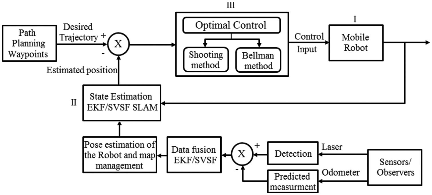
State estimation EKF/SVSF-SLAM and optimal control for mobile robot.
This article is organized as follows. Section “Process model of UGV” depicts the process model of UGV. In section “EKF-SLAM algorithm,” the EKF-SLAM algorithm is detailed and compared with the proposed SVSF-SLAM algorithm. The implementation of this latter is presented in section “SVSF-SLAM algorithm.” In section “Optimal control,” we describe path planning with optimal control. Finally, results and discussion are provided in section “Results and discussion” followed by conclusion and perspectives.
Process model of UGV
The Pioneer

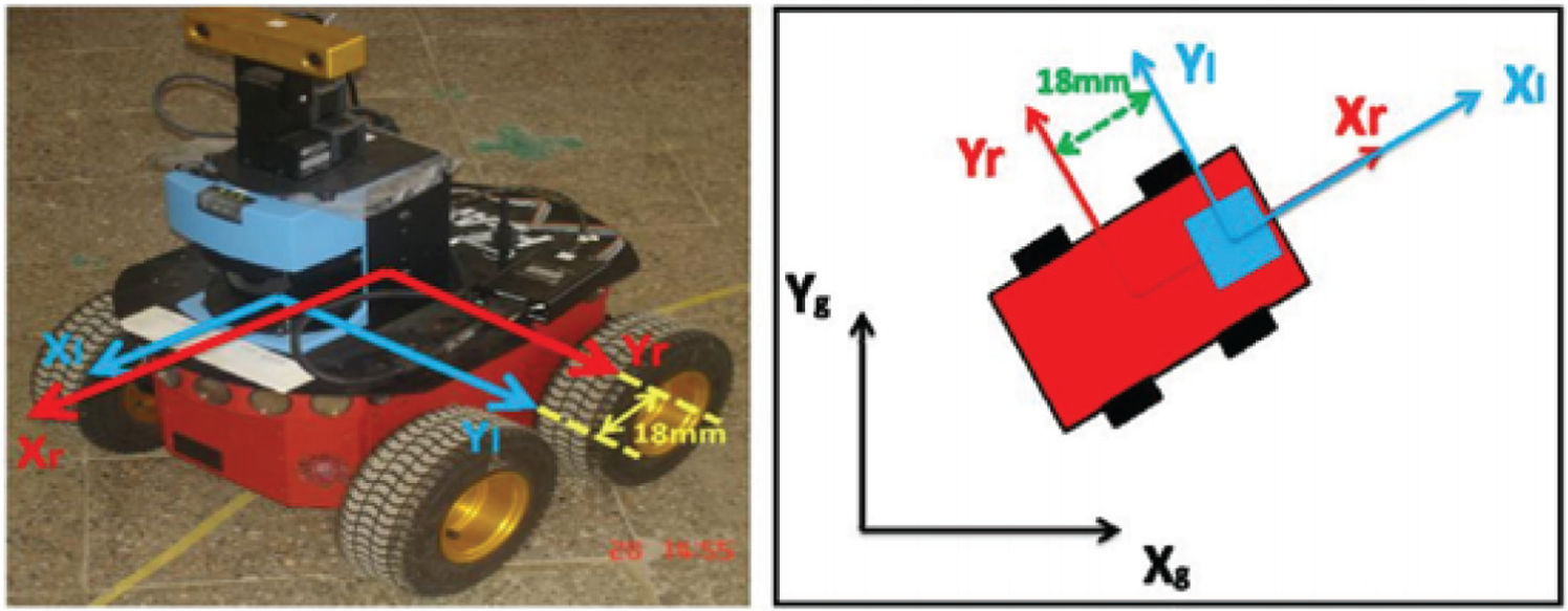
Mobile robot (P3-AT) Robotic Laboratory—EMP.

SICK 2D laser range finder (LMS-200).
From Figure 4 and Sfeir, 15 the state transition equation of the robot is given by

where
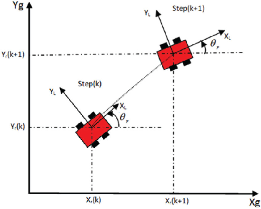
Kinematic model of the UGV.
When

The odometry depends on the assumption which is only true if there is no slipping in the robot’s wheels. The angular velocity delivered by the gyroscope can be integrated to provide the orientation (
When


Direct observation point–based model
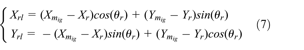
The representation of point coordinates in the global frame according to its coordinates in the local frame is given by 20

The overall transformation to local inverse model is given as follows
where
The subscript

where
Inverse observation point–based model
The landmark mapping model is an inverse observation model. Knowing the robot state and the landmark coordinate, the inverse observation model


where
Direct observation line–based model
The direct observation model is given by20,23

Inverse observation line–based model
The mapping model is an inverse observation model

There are many types of features association “line to line,”24,25“point to line,” 26 and “point to point.”24,27 In this article, we will do a comparative’s survey between two types of association “point to point” and “line to line.” Since the processing time of the EKF/SVSF-SLAM approach “point to point” is very important and allocates a large memory space, thus, in the association step, we propose to use a method based on “line to line” that is quicker than the standard “point-to-point” approach. In our work, we used the method “Split and Merge” which is largely used for line extraction.24,25
EKF-SLAM algorithm
The discretization form of the system and nonlinear model measurement used for state estimation can be written as follows


The EKF provides an approximation of the optimal estimate.
Initial estimates for
Project the state

Prediction
Project the error covariance ahead. The prediction covariance matrix

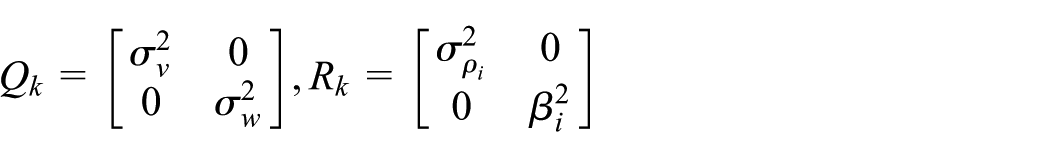
where

where

Observation and update
Linearization of the observation model

The update cycle of the Kalman filter is applied to
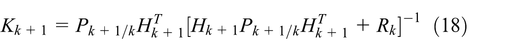
Compute the Kalman gain
Update estimate with measurement

Update error covariance

Even as the environment is investigated, new features are detected and should be put on the accumulation map. In this case, the state vector and the output error estimate matrix are calculated from the new observation.
Map management
Add
Initialization of the covariance matrix

where

and

Initialization of the inter-covariance matrix

Increment the state vector

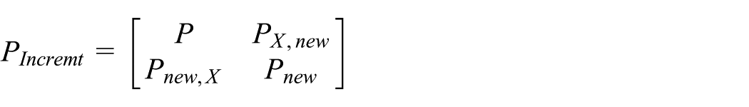
Increment the covariance matrix
SVSF-SLAM algorithm
The variable structure filter (VSF) was created in 2003, as a new estimator using a sliding mode concept where switching gain is used to ensure that the estimates converge to true state values. 30 As shown in Figure 5, the SVSF utilizes a switching gain to converge the estimates to within a boundary of the true state values (i.e. existence subspace).31,32

SVSF estimation concept.
A corrective term, referred to as the SVSF gain, is computed as a function of the error in the predicted output, as well as a gain matrix and the smoothing boundary layer width.30,32,33 The corrected term calculated in equation (21) is then used in equation (24) to find a posteriori state estimate. The priori and posteriori output error estimates are considered as critical variables which are defined by equations (25) and (26), respectively32,33 The estimation progression makes a summary of equations (21)–(28) and is repeated iteratively.

where ∘ represents “Schur” element-by-element multiplication; + refers to the pseudo inverse of a matrix;

This equation
with

The update of the state estimates can be calculated as follows

The priori and posteriori output error estimates are defined as follows


The SVSF filter provides a robust and stable estimate to modeling uncertainties and errors.31,33
The calculation of the SVSF gain is needed to use two main parameters. The first parameter is

As maintained by Sfeir, 15 the estimation process is stable and converges to the existence subspace if the following circumstances are contented 31

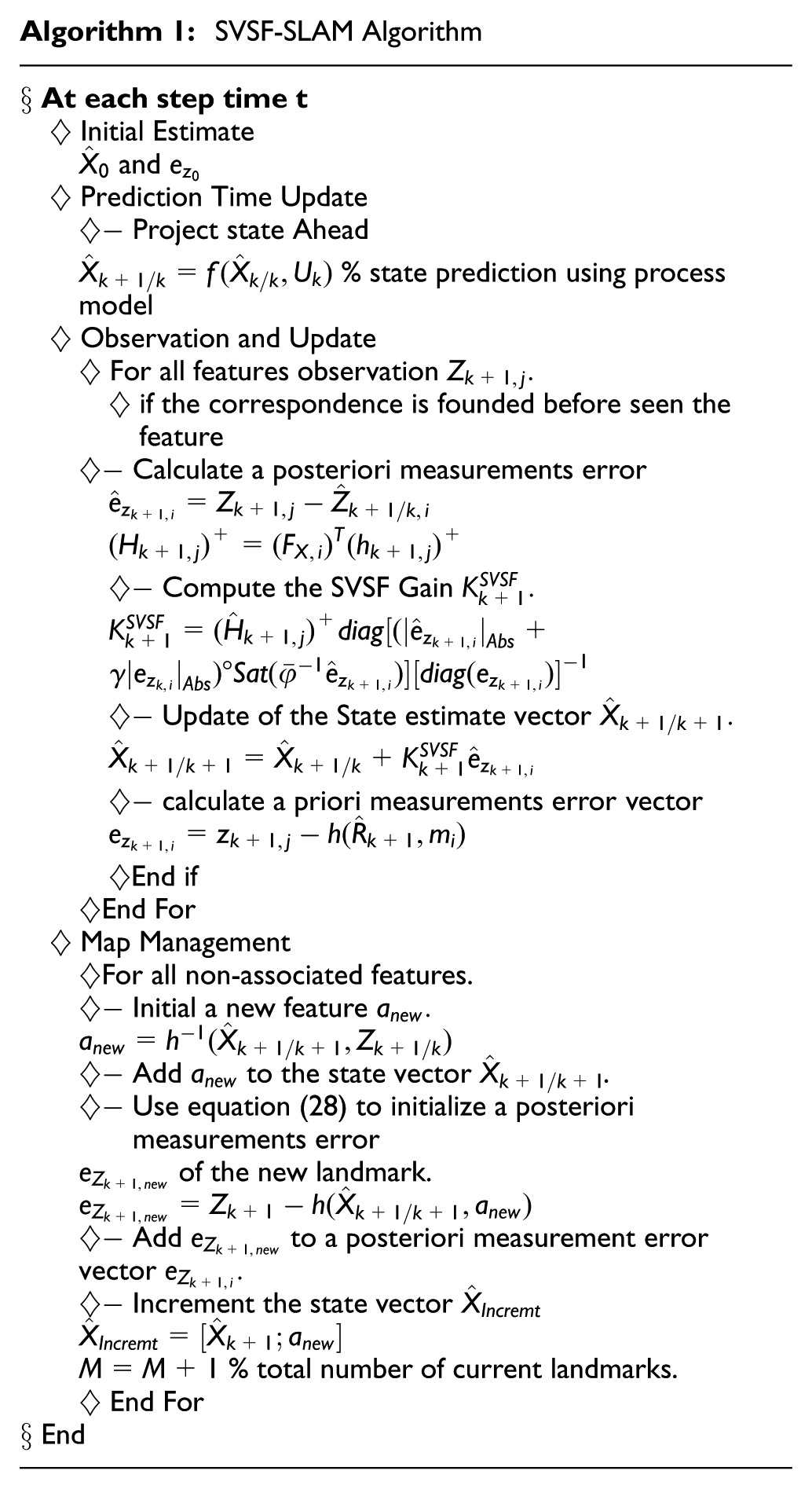
Two association approaches are proposed: “point to point” and “line to line.” The steps of SVSF-SLAM algorithm is illustrated in the algorithm 1.20,22 In this work, we also treat the problem of optimal control, focusing on two main methods which have proven to be effective on mobile robots: the Shooting and Bellman methods.

Steps of the EKF/SVSF-SLAM principle.
Optimal control
In this section, we provide a path planning algorithm based on optimal control theory. In the beginning, we use the Shooting methods based on the Pontryagin’s principle.16,34 In this principle, we determine an optimality equation, that is, a differential algebraic equation system is provided with an initial condition and a final condition and the adjoint equations. In other words, we should note that in the adjoint equation, derived from the Pontryagin’s principle, no information is given concerning the initial or the final conditions. Consequently, this equation is hard to be used numerically. Thus, in order to determine the initial condition of the adjoint state, we use the Shooting indirect method for the numerical procedure. 34 After this, we present the results of numerical experiments implemented using MATLAB facilities. For classical method problems, the solution can be obtained analytically or numerically. On the other hand, we use the Bellman principle which is the direct method and gives an appropriate condition to the optimality solution.35–37
Numerical solution with the Shooting method
The optimal control problem of the robot is stated as follows: Find the control

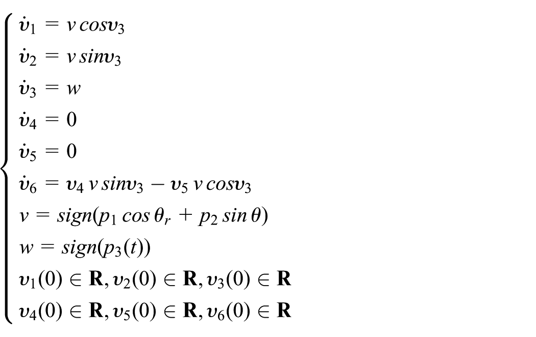
subject to the differential constraints

The prescribed boundary conditions
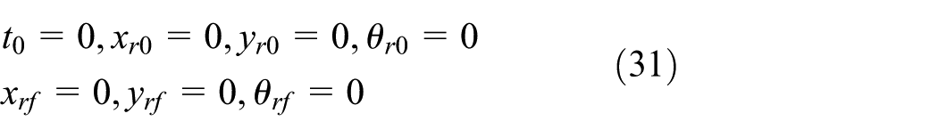

Equation (29) is equivalent to

The Hamiltonian is given by

The Euler–Lagrange equations are given by


From Hamiltonian

The following equation is given to find a control

then

Consequently, we deduce

In the numerical solution, we used the Shooting indirect method to determine a final time. Then we have to solve the following system
Let
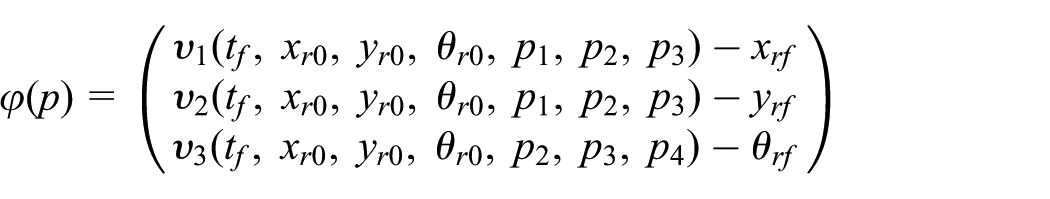
Solving the problem, we can write: Find
The integration algorithm of a differential system with initial condition (i.e. the Euler or Runge–Kutta procedure) to compute the Shooting function
The solution algorithm
Numerical solution with the Bellman method
In this section, we use the Bellman principle to solve the same system with free final time which is the direct method. We consider the control of a discrete time dynamical system

where

where

where

where
Results and discussion
SLAM results
Simulation results
The simulation results of the proposed SVSF-SLAM algorithm for UGV localization problem are presented. The results of our proposed algorithm are compared with EKF-SLAM algorithm. The sampling rates used for each filter and sensors used in this study are as follows 20

Figure results which are presented show the estimated position of the UGV using EKF and SVSF, with
Test 1: zero-mean Gaussian noise
In the first experiment, we use a white centered Gaussian noise for process and observation model where

Test 2: colored noise
In this experiment, we use a white noise with bias for process and observation model where

Figure 7 shows proposed algorithms and provide accurate positions when process and measurement noise are zero-mean and Gaussian. The position errors are shown in Figure 8. We note that the EKF-SLAM algorithm gives higher quality in estimation error terms compared with SVSF-SLAM algorithm. At 1550 iteration, we note significant increase of the SVSF-SLAM algorithm consistency in comparison to EKF-SLAM algorithm caused by closing-loop detection. The robot closes the loop making the error in the environment to decrease at 1550 iteration when it frequently moves into pre-visited regions.

Pose estimation with zero-mean Gaussian noise.

Error position of the robot with zero-mean Gaussian noise.
In the first test, by looking at the root mean square error (RMSE) of EKF/SVSF-SLAM algorithms, within the sight of zero-mean Gaussian noise, we can show that the EKF notices better results with zero-mean Gaussian noise. This can be found in Figure 9. EKF-SLAM algorithm gives the best position results and is more accurate than SVSF-SLAM algorithm. This can be translated as follows: In this case, the EKF gives a good accuracy when the process and observation noise are uncorrelated zero-mean Gaussian with known covariance. On other hand, when the control noise is colored, the EKF-SLAM algorithm is unsuccessful with high error in comparison to the SVSF-SLAM algorithm. For this situation, the map created by the proposed SVSF-SLAM algorithm with colored noise is not debased in quality as can be seen in Figure 10.

Position RMSE under zero-mean Gaussian noise.
Pose estimation with colored noise.
The position errors are appeared in Figure 11, we note that the SVSF-SLAM algorithm performs altogether superior to the EKF-SLAM algorithm in terms of estimation error. The SVSF is in a position to get the best of information in a short time and come up with a relatively estimate.

Error position of the robot with colored noise.
Figure 12 puts in view the evaluation results of an investigation in comparison to the convergence RMSE of both algorithms. As for the results of the second experiment in comparison to the RMSE of EKF/SVSF-SLAM algorithms, in appearance of colored noise, we note that the RMSE showed the best outcomes with colored noise as can be seen from Figure 12. SVSF-SLAM algorithm is more accurate than EKF-SLAM algorithm in terms of position.

Position RMSE under colored noise.
The structure of SVSF-SLAM algorithm reveals that it reduces the computational complexity of the algorithm. One inconvenient of the EKF-SLAM algorithm is the use of the full dimension of the state vector to update the pose and the map estimation. In this way, the computation time will increment with the size of the state vector. On the other hand, the SVSF-SLAM algorithm uses just the posture of UGV and the current feature to update the map and the pose estimation which makes the computational time independent of the size of the state vector. The SVSF-SLAM algorithm remains nearly constant per iteration depending on the number of visible landmarks (Figure 13).
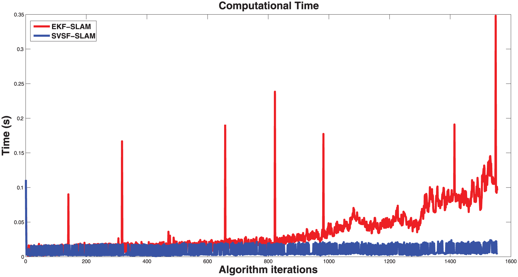
Computational time comparison.
Experimental results
Figure 14 shows the visited places (three (03) rooms (see (a), (b), and (c)) + corridor (see (d)) of the building (indoor environment). We made a trip over a distance of

Shots of visited places.
When the robot moves in the map, it uses a laser to detect landmarks such as points and lines. In this experiment, the maximum range of the SICK laser is
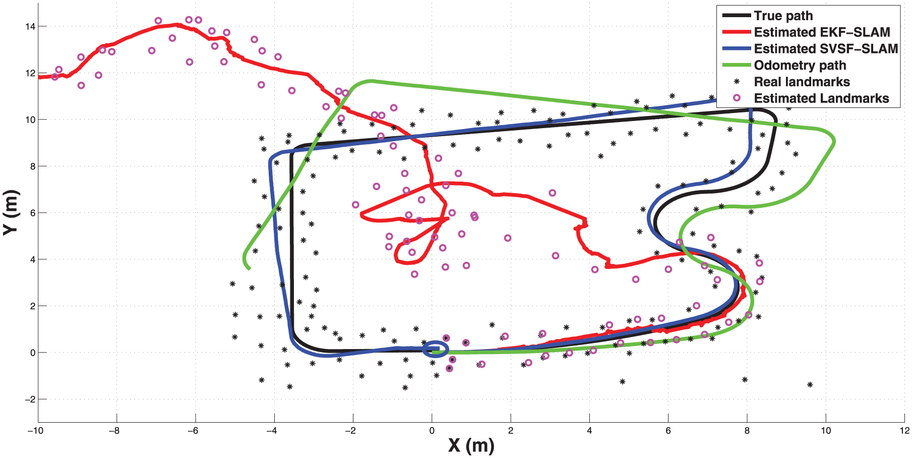
Trajectory estimated by the SVSF-SLAM algorithm, as shown in Figure 15, is more accurate in comparison to the EKF-SLAM algorithm. The SVSF-SLAM algorithm provides the best position in comparison to the EKF-SLAM algorithm. The SVSF-SLAM algorithm shows that our results are consistent and realistic in comparison to the EKF-SLAM algorithm. We see clearly as shown in Figure 15(a) that the pose errors of the EKF-SLAM algorithm increase significantly and the robot is so far and does not arrive to the initial position because of the previous errors made through its trajectory. Moreover, from Figure 15(b), at the final time, we can remark that the robot detects a common feature which improves the consistency of the SVSF-SLAM as well as the EKF-SLAM algorithm.
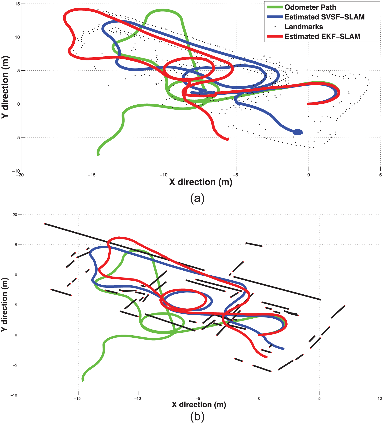
Result of SVSF/EKF-SLAM algorithms based on point and line approaches in real time.
From the starting position to the final position (loop closure at
The structure of the SLAM algorithm–based line has been shown to decrease the computational time in comparison to the SLAM algorithm–based point which is proportional to the state vector length. EKF-SLAM algorithm allocates a large memory space and requires heavy significant computational time (see Figure 16).

Computational time of EKF/SVSF-SLAM algorithms based on point and line approaches in real time.
In this environment, we note that the path given by the odometer is completely drift and this is due to the great range done by the robot. Besides, the SVSF-SLAM algorithm is better than EKF-SLAM algorithm. According to these results, we can confirm how a better localization of the robot makes the possibility of a coherent environment map building (see Figure 15).
Optimal control results
The path planning with optimal control
We have implemented the methods (Shooting and Bellman) using EKF/SVSF-SLAM localization. Table 1 depicts the results of the two methods we used to solve the SLAM localization. Numerical solution provides the following results with the Shooting and Bellman methods. To improve the position accuracy of the numerical solution of optimal control problems, we use the Bellman method compared to the Shooting method which has low accuracy and decreases the convergence of the robot position. We compare the true positions (Table 1) with the results given by the Shooting and Bellman methods (Tables 2 and 3), (Tables 4 and 5), and (Tables 6 and 7), respectively.
True and estimated positions for all different trajectories (EKF/SVSF-SLAM and odometer).

The Shooting method (SVSF-SLAM).

The Bellman method (SVSF-SLAM).

The Shooting method (EKF-SLAM).

The Bellman method (EKF-SLAM).

The Shooting method (odometer).

The Bellman method (odometer).

Through the two methods, best results are obtained by SVSF-SLAM compared to EKF-SLAM and the odometer; moreover, short time is required by the proposed approach (see Table 8). We can say that the result sets using the Bellman method are much better than the Shooting method. The Shooting method is not accurate compared to the Bellman method, because the initial conditions of adjoint state are sensible, that make us away from the correct positions. The solution for SLAM problem and the accuracy of the result are controlled by the accuracy of the Bellman method used as opposed to the Shooting method with the use of the Euler–Lagrange equations. The following figures show the results of optimal control with the Shooting and Bellman methods.
Final time with the Shooting and Bellman methods for three methods (EKF-SLAM, SVSF-SLAM, and odometer).

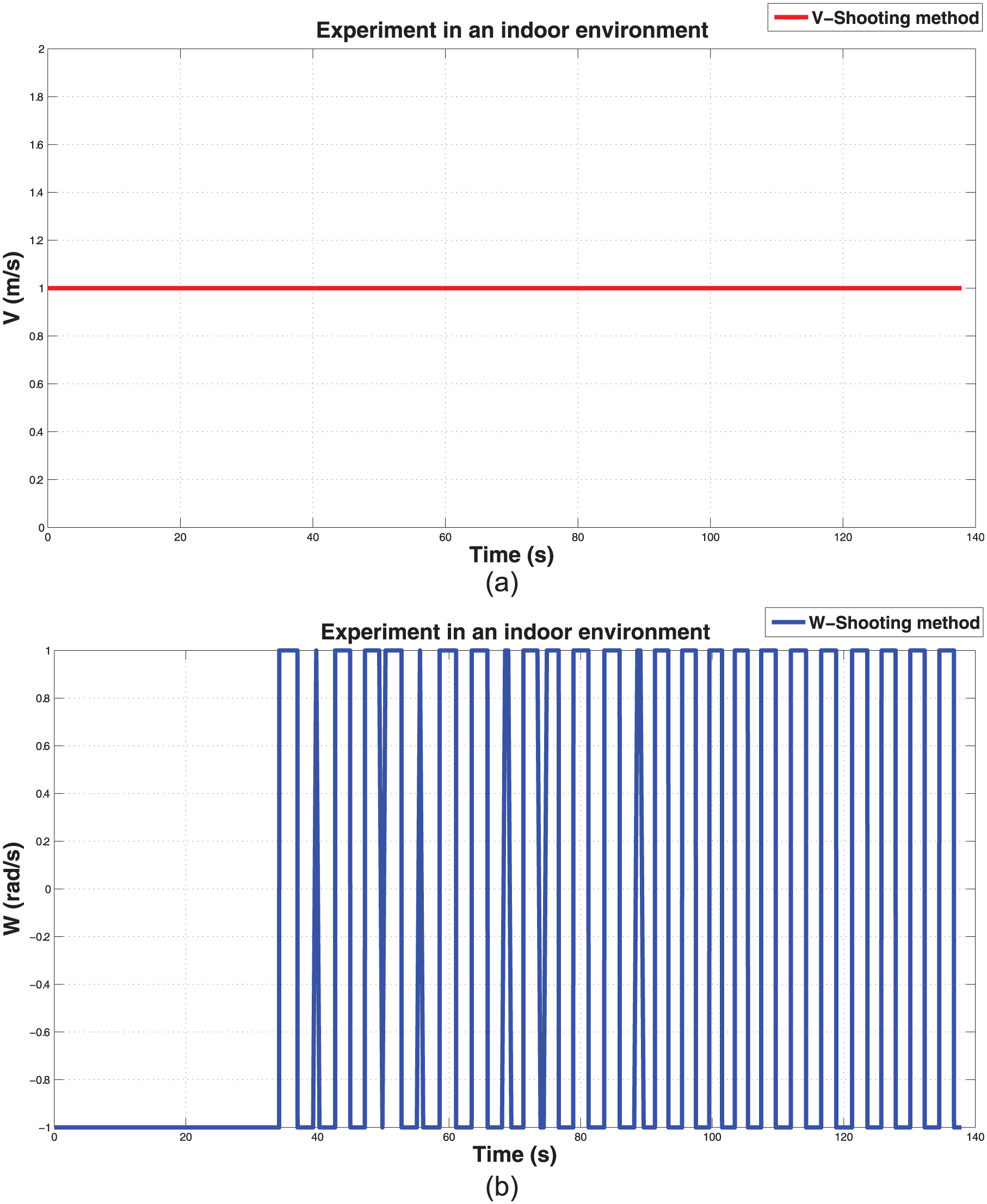
The final time is the minimum time to come to the last time point corresponding at 155.1 s (final time) to the final position (0,0,0). From Table 9, note that the final time found by the Bellman method is better than the Shooting method. As can be seen from Table 8, the minimal final time is given with SVSF-SLAM localization. Then, we compared the true positions of our experiments for different positions of localization such as SVSF, EKF, and odometer. We determined the robot controls for each localization of two methods and we made a comparison between them. We notice that the robot control parameters using the Bellman method is better than Shooting method that the SVSF-SLAM localization is used. The results conform with our data (see Figures 17–19).
Final time with the Shooting and Bellman methods for three methods (EKF-SLAM, SVSF-SLAM, and odometer).


Control of V and W in an indoor environment–based point (SVSF-SLAM/EKF-SLAM/odometer).
Control of V and W with the Shooting method in an indoor environment–based point (SVSF-SLAM).

Control of V and W with the Bellman method in an indoor environment–based point (SVSF-SLAM).
From Figures 20 and 21, we noted that the results found using the Bellman principle are much better than the Shooting method, and the points

Control optimal of UGV with the Shooting method: SVSF-SLAM, EKF-SLAM, and odometer.

Control optimal of UGV with the Bellman method: SVSF-SLAM, EKF-SLAM, and odometer.

Comparison of the Shooting and Bellman methods.

Control of V with the Shooting and Bellman methods (EKF-SLAM).

Control of W with the Shooting and Bellman methods (EKF-SLAM).

Control of V with the Shooting and Bellman methods (SVSF-SLAM).
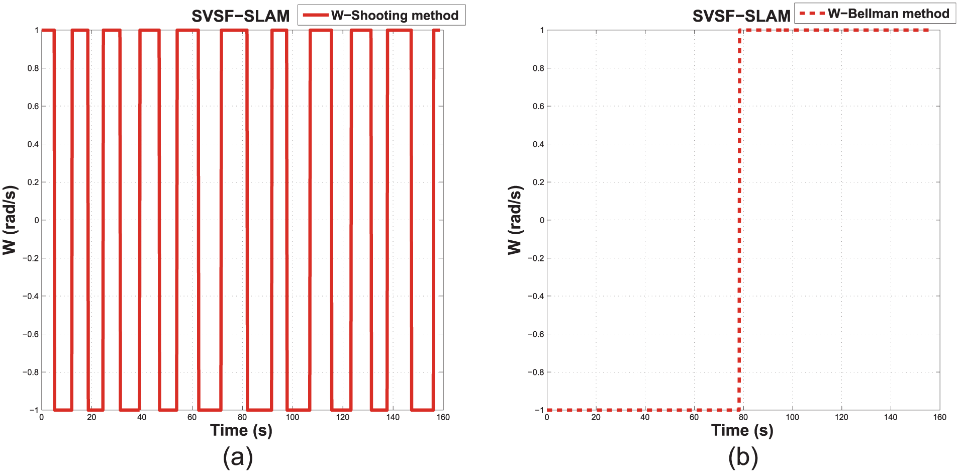
Control of W with the Shooting and Bellman methods (SVSF-SLAM).

Control of V with the Shooting and Bellman methods (odometer).

Control of W with the Shooting and Bellman methods (odometer).
Table 9 shows the energy of the robot orientation
Conclusion
In this article, SLAMPP algorithm have been proposed for UGV navigation. As this UGV operates at low speed, path planning and optimization strategies are developed without considering vehicle dynamics. Only the kinematics of the vehicle and the environment constraints are considered.
Based on SVSF-SLAM algorithm localization and optimal control theory, the proposed algorithm (SLAMPP) improves the path in terms of continuity by providing a smoother and more comfortable trajectory tracking. In addition, the proposed algorithm requires less computation time to achieve the improvement. The proposed approach is validated using simulation and experimental data. Several experiments are tested under realistic conditions and good performances are obtained by the SVSF-SLAM compared to the EKF-SLAM algorithm. As perspectives, we propose to extend the proposed approach for multiple robots (UGVs, UAVs, and AUVs).
Footnotes
Handling Editor: Francesco Massi
Declaration of conflicting interests
The author(s) declared no potential conflicts of interest with respect to the research, authorship, and/or publication of this article.
Funding
The author(s) received no financial support for the research, authorship, and/or publication of this article.