Sage Journals: Discover world-class research

Abstract

In this article, a mathematical model of hydrodynamic force was established to model the influence of wall in realizing the precise control and maneuverability of a complex-shaped underwater robot. A hydrodynamic model of a robot for use in a nuclear reaction pool was presented containing not only hydrodynamics coefficients but also a wall hydrodynamic force term, which was often ignored for robots used at sea. First, hydrodynamic coefficients in the model, including viscous and inertial coefficients, were solved by simulating steady-state and unsteady-state motion by computational fluid dynamics. Next, the wall hydrodynamic force was calculated by computational fluid dynamics for different velocities and distances from the wall, and the scope of influence of the wall was identified. Finally, hydrodynamic coefficients without the wall effect and with the wall hydrodynamic force under different conditions were measured experimentally in a circulating water tank. The result demonstrated the accuracy of hydrodynamic calculation by computational fluid dynamics and verified the reliability of the hydrodynamic mathematical model.

Keywords

Underwater robot hydrodynamic coefficients computational fluid dynamics wall effect a prototype test

Introduction

In recent years, nuclear energy industry was rapidly developed around the world. After the Fukushima nuclear accident in Japan, nuclear security issues were paid worldwide attention to.^1,2 Many research institutes have devoted considerable effort to research on nuclear rescue robots.^3,4 We have developed an underwater robot with a welding device that can weld a nuclear reaction pool in an emergency. The semi-autonomous underwater unmanned robot can not only be manually operated through an umbilical cable but also independently patrol near the operation target. The design of the robot’s controller and the analysis of its maneuverability are based on a dynamic model. In this approach, a mathematical model of hydrodynamic force⁵ treated as a disturbance factor is a main component of the dynamics to improve control precision. Hence, the analysis of the hydrodynamic characteristics is significant. Additionally, when moving while attached to wall to weld or inspect, the hydrodynamic force will be altered due to the wall obstruction.⁶ Therefore, the hydrodynamic model presented here includes not only hydrodynamic coefficients but also a hydrodynamic force term due to the blocking effect of the wall.

At present, there are three methods to calculate hydrodynamic coefficients: estimation of an empirical formula, testing a restraint model, and numerical simulation.⁷ The empirical formula method simplifies the robot as a combination of various geometries. It is effective in solving the hydrodynamic force on a robot with a simple structure,^8,9 but the calculated result is imprecise for a robot of complex structure, so this method is seldom used. The restraint model test method is suitable for solving hydrodynamic coefficients of all types of underwater robots. In recent years, many scholars have published much research.^10–14 Although this method is most effective, it has failed to become widely popular because of its long test periods and high cost. With the development of computer technology and computational fluid dynamics (CFD) technology, numerical simulation^15–17 with short cycles, low cost, and manpower savings has become a new method for determining hydrodynamic coefficients. Recently, this method has been widely used to achieve research results. Tyagi and Sen,¹⁸ Cheng and Lau,¹⁹ and Wu et al.²⁰ presented a method to determine the damping coefficients by an experiment to verify the theoretical model obtained from CFD. The added mass coefficients were solved by simulating the planar motion mechanism test and a free-decaying test in CFD from the literature.^21–24 A method of solving the hydrodynamic coefficients of a complex-shaped robot was proposed, and the authenticity of the simulation was verified by an experiment in Tang et al.²⁵ With robot motion near a wall, the hydrodynamic force due to the blocking effect of a wall is called the wall hydrodynamic force. In previous research, there was not much research on the influence of wall effect for robots. Du et al.²⁶ analyzed the change in hydrodynamic force close to the sea bottom. Suzuki et al.²⁷ obtained a linear relationship between a vertical hydrodynamic force and the distance from the sea bottom with a model test. Zhu et al.²⁸ analyzed the relationship between resistance, lift coefficients, and the distance from the bottom when robot moved linearly. Zou and Larsson²⁹ presented a CFD method to calculate the effect of a bank on ship under different conditions.

Although these reports have worked out theoretical hydrodynamic models by solving hydrodynamic coefficients, the underwater robots are used in the sea, namely, the open water domain. In these scenarios and models, the blocking effect of a wall on an underwater robot is ignored. Recently, some literature discusses the effect of a wall on a robot by the numerical simulation, but only qualitatively; the effect has not been quantified until now. Moreover, there is no experiment designed to measure the wall hydrodynamic force to verify the accuracy of the simulation. In this work, to quantify and predict the effect of the hydrodynamic force on an underwater robot with a motion near the wall, the CFD method and a prototype test are used. First, a theoretical model of the hydrodynamic force resulting from the blocking effect of walls is presented in the horizontal and vertical planes. Then, the wall hydrodynamic force is solved by a method similar to a steady motion simulation by CFD. Finally, a hydrodynamic test is designed in a circulating water tank to verify the accuracy of the results of the wall hydrodynamic force obtained by CFD, and for difference flow velocities the influence scopes of the wall are obtained. The work conducted in this article establishes a precise mathematical model and is helpful for the control designer and maneuverability research.

This article is organized as follows. Section “Structure and function of robot” describes an underwater robot to weld and inspect the wall of a nuclear reaction pool. Section “Hydrodynamic model” presents a mathematical model of the hydrodynamic force with a robot motion near the wall in the horizontal and vertical planes. Section “Hydrodynamic coefficients solved by CFD” reports a steady and unsteady motion simulation in CFD to solve the viscous and inertial hydrodynamic coefficients in the model. Section “Wall hydrodynamic force solved by CFD” depicts a method of solving the wall hydrodynamic force by CFD. Section “Prototype test” describes a prototype test including a direct resistance test, an oblique towing test, a planar motion mechanism test, and a wall hydrodynamic test. Finally, some conclusions are drawn.

Structure and function of robot

In previous research, many underwater robots have been designed. Liu et al.³⁰ designed a new multi-functional and model-switched remotely operated vehicle for decontamination of underwater structures at sea. Miao and Pang³¹ presented a small inspection-class underwater robot that carried a video camera for underwater inspection. Anwar et al.³² designed a portable low-cost remotely operated underwater vehicle that can conduct surveys in shallow waters.

These previous robots were used only to observe in water; they could not perform complex tasks. In this section, the research object is an open-frame underwater robot equipped with a welding device and an observation device; it can weld the wall of a nuclear reaction vessel in an emergency and perform a daily inspection. The size of the framework of the robot (Figure 1), which is made of Teflon, is 1.06 m × 0.65 m × 0.66 m (length × width × height). The drainage volume of the body is ΔV = 0.21 m³, and its mass is = 117 kg. Pressurized cabins for power and control are arranged on the body. A welding torch and a camera are installed on a 3-degree-of-freedom (DOF) movement platform on the body. There are eight propellers on the body, which are the only power output devices equipped. The maximum thrust and power of every propeller are, respectively, 50 N and 300 W. The propellers are divided into two layers: four propellers on the top layout provide power for heave, roll, and adsorbing on the wall; the others on the bottom layout allow the body to surge, sway, and yaw.

Figure 1.

A prototype of an underwater robot.

The body can roll 90° about its x-axis to address and patrol on a side wall, as the torch has a downward direction. Buoyancy material is installed on the bottom of the body to reduce the metacentric height, which can reduce restoring moment to enable the device to roll. The structure of the robot is symmetrical in x-axis and y-axis directions; hence, the distance between them is 8 mm in z-axis direction and 0 mm in x-axis and y-axis directions.

Hydrodynamic model

To facilitate describing the movement of the robot, a fixed coordinate frame E-ξηζ and a moving coordinate frame O-xyz are established as shown in Figure 2. The origin of the moving coordinate frame coincides with the center of mass of the robot. The linear velocities in the longitudinal, transverse, and vertical directions are, respectively, represented by u , v , and w ; the roll, pitch, and yaw angular velocities are expressed as p , q , and r ; the force are represented by a matrix $τ = [X, Y, Z, K, M, N]^{T}$ .

Figure 2.

Fixed and moving coordinate systems of robot.

The blocking effect of the water against the robot’s movement is called as the hydrodynamic force. Hence, hydrodynamic force is a function of motion parameters. According to their origin, the hydrodynamic forces can be classified into inertial and viscous hydrodynamic forces. Additionally, a wall hydrodynamic force is presented due to the blocking effect of the wall when robot moves near the wall.

From the literature,³³ a hydrodynamic model of a robot moving in the horizontal plane is established in view of the impact of the wall as follows

X_{H} = X_{\overset{\cdot}{u}} \overset{\cdot}{u} + X_{uu} u^{2} + X_{vv} v^{2} + X_{rr} r^{2}

(1a)

Y_{H} = Y_{\overset{\cdot}{v}} \overset{\cdot}{v} + Y_{\overset{\cdot}{r}} \overset{\cdot}{r} + Y_{v | v |} v | v | + Y_{v} v + Y_{r | r |} r | r | + Y_{r} r + R_{YH}

(1b)

N_{H} = N_{\overset{\cdot}{v}} \overset{\cdot}{v} + N_{\overset{\cdot}{r}} \overset{\cdot}{r} + N_{v | v |} v | v | + N_{v} v + N_{r | r |} r | r | + N_{r} r + R_{NH}

(1c)

Similarly, the hydrodynamic model when robot moves in the vertical plane is

\begin{matrix} X_{V} = X_{\overset{\cdot}{u}} \overset{\cdot}{u} + X_{\overset{\cdot}{q}} \overset{\cdot}{q} + X_{u} u + X_{w} w \\ + X_{q} q + X_{uu} u^{2} + X_{ww} w^{2} + X_{qq} q^{2} \end{matrix}

(2a)

\begin{matrix} Z_{V} = Z_{\overset{\cdot}{w}} \overset{\cdot}{w} + Z_{\overset{\cdot}{q}} \overset{\cdot}{q} + Z_{w} w + Z_{w | w |} w | w | + Z_{q} q \\ + Z_{q | q |} q | q | + Z_{ww} w^{2} + Z_{qq} q^{2} + R_{ZV} \end{matrix}

(2b)

\begin{matrix} M_{V} = M_{\overset{\cdot}{u}} \overset{\cdot}{u} + M_{\overset{\cdot}{w}} \overset{\cdot}{w} + M_{\overset{\cdot}{q}} \overset{\cdot}{q} + M_{w | w |} w | w | \\ + M_{w} w + M_{q | q |} q | q | + M_{q} q + M_{ww} w^{2} \\ + M_{qq} q^{2} + R_{MV} \end{matrix}

(2c)

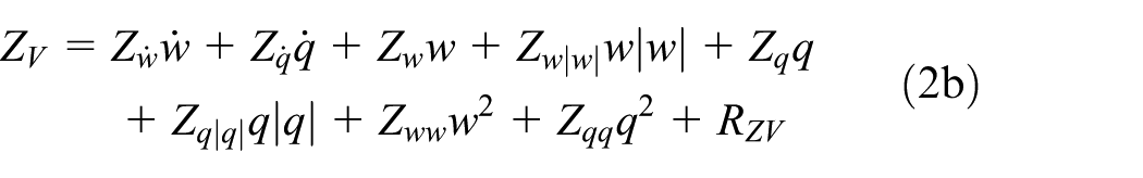
where inertial hydrodynamic coefficients are expressed as $X_{\overset{\cdot}{u}}, Y_{\overset{\cdot}{v}}, Z_{\overset{\cdot}{w}}, \dots$ , linear viscous hydrodynamic coefficients are $Y_{v}, Z_{w}, K_{p}, \dots$ , nonlinear viscous hydrodynamic coefficients are $Y_{v | v |}, Z_{w | w |}, K_{p | p |}, \dots$ , and the second-order viscous hydrodynamic coefficients are represented by $X_{uu}, X_{vv}, X_{rr}, \dots$ . When moving in the horizontal plane, the wall hydrodynamic forces are expressed as $R_{YH}, R_{NH}$ ; moving in the vertical plane, they are expressed as $R_{ZV}, R_{MV}$ .

The hydrodynamic coefficients in formulas (1) and (2) are dimensional, and their values are easily influenced by the model’s scale, and so on. To overcome these effects, the coefficients are re-defined as dimensionless according to the similarity principle. Therefore, the coefficients of forces proportional to the velocity are dimensionless by $1 / 2 ρ l^{2} \sqrt{gl}$ , which are proportional to the square of the velocity by $1 / 2 ρ l^{2}$ . Here, l is the model length, ρ is the water density, and g is the gravitational acceleration. The coefficients of moments proportional to the velocity are obtained by $1 / 2 ρ l^{3} \sqrt{gl}$ , and the moment coefficients are proportional to the square of the velocity by $1 / 2 ρ l^{3}$ .

Hydrodynamic coefficients solved by CFD

In this section, hydrodynamic coefficients in formulas (1) and (2) will be solved by numerical simulation and an estimating formula.³⁴ The numerical simulation can be divided into two types: an unsteady-state simulation and a steady-state simulation.

Before calculating CFD, a calculation domain divided into internal and external flow fields is established as shown in Figure 3. An external flow field of the domain was like a cube region, the size of which was 11L ×9L × 9L (L was the length of robot). The size of an internal flow field which was also cubic was 2L × L × L. The boundary of the internal flow field extending back a distance of 6L was the inlet boundary of the external flow field, and extending forward a distance of 3L was the outflow boundary of the external flow field, and extending to the left, right, top, and bottom a distance of 4L were other boundaries of the external flow field.

Figure 3.

A computational domain in CFD.

The calculation domain was then meshed. Here, a multi-block meshing strategy was used due to the complex shape of the body, namely, an unstructured tetrahedron grid that can best adapt to the complex shape of the robot and for which it was easy to control the size of nodes and the grid density in the internal flow field; the external flow field used a structured hexahedral mesh to reduce the number of mesh points, which can improve calculation efficiency. The total mesh size of the computational domain was about 741,900.

The entrance of the external flow field was set as an inlet velocity condition, and the exit was set as an outlet pressure condition. The other boundaries of the external flow field were set as free-slip walls. The surface of the model was set as a no-slip wall.

In CFD, some parameters were set as following: the turbulence model was set as standard k-epsilon with standard wall function; SIMPLE algorithm was used to calculate pressure–velocity coupling; pressure discretization was the first-order upwind discrete mode; and momentum discretization, turbulent kinetic, and turbulent dissipation rate were the second-order upwind discrete mode. Under-relaxation factors of pressure, momentum, turbulent kinetic energy, turbulent dissipation rate, and turbulent viscosity were 0.5.

Unsteady motion simulation test

An unsteady motion simulation was conducted to solve for inertial hydrodynamic coefficients. The planar motion mechanism was simulated virtually by CFD, namely, the robot made motions such as pure heave motions, pure pitching motions, pure sway motions, and pure rolling motions, using user-defined functions (UDFs). The hydrodynamic force was solved with longitudinal flow acting on the body. The process of solving for the inertial hydrodynamic coefficients was described taking the simulation of the pure heave motion of the robot as an example.

In the computational domain, the pure heave motion equation of the robot was

{\begin{matrix} ζ = a \sin ω t \\ \overset{\cdot}{ζ} = w = a ω \cos ω t \\ \overset{\cdot\cdot}{ζ} = \overset{\cdot}{w} = a ω^{2} \sin ω t \end{matrix}

(3)

where the amplitude of robot motion was a = 0.04 m; the vertical displacement was expressed as ζ; the vertical velocity and acceleration of the robot were, respectively, $w$ and $\overset{\cdot}{w}$ ; and the angular frequency was ω.

The grid nodes in the internal flow field will experience sinusoidal movement according to formula (3) by UDF; the hydrodynamic forces were calculated under conditions in which the oscillation frequencies were set at f = 0.2, 0.25, 0.3125, 0.4, 0.5, and 0.625 Hz. A stable plot of dimensionless force versus time can be obtained after six to seven calculation cycles. A set of discrete points at time t was obtained, which can be written as a first-order Fourier series

f (t) = \frac{a_{0}}{2} + a_{1} \cos ω t + b_{1} \sin ω t

(4)

namely

{\begin{matrix} Z' = Z_{a} \sin ω t + Z_{b} \cos ω t + {Z'}_{0} \\ M' = M_{a} \sin ω t + M_{b} \cos ω t + {M'}_{0} \end{matrix}

(5)

assuming

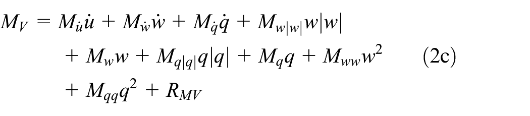
\begin{matrix} Z_{a} = - \frac{a ω^{2} L}{V^{2}} Z'_{\overset{\cdot}{w}}, Z_{b} = \frac{a ω}{V} Z'_{w}, \\ M_{a} = \frac{a ω^{2} L}{V^{2}} M'_{\overset{\cdot}{w}}, M_{b} = \frac{a ω}{V} M'_{w} \end{matrix}

(6)

where L represents the characteristic length of the robot and V represents the characteristic velocity.

From formulas (4)–(6), the coefficients Z_a, Z_b, M_a, and M_b were solved by the Fourier expansion method in MATLAB, followed by the hydrodynamic coefficients related to the pure heave motion.

Steady-state motion simulation

The simulation experiment of steady-state motion included a linear motion simulation and an oblique motion simulation.

The robot was placed in the calculation domain with no pitching and rolling angle when launching a linear motion simulation. The velocity of the robot was kept constant in a straight line under a rated speed that the robot reached after acceleration from rest at 0.1 m/s² by UDF. The resistance was calculated at different rated speeds. Here, the rated speed varied from 0.1 to 0.8 m/s in increments of 0.1 m/s.

The oblique motion simulation was developed in the vertical and horizontal planes. The calculation was illustrated taking the oblique test in the horizontal plane as an example. The flow velocity at the entrance to the computational domain was kept constant; the angle between the velocity direction and ξ-axis in fixed coordinates was an angle of drift that was positive if the rotation from the velocity direction to the ξ-axis was clockwise. Here, the hydrodynamic force and moment were calculated with the angle of drift varying from −10° to 10° in increments of 2°. The hydrodynamic coefficients related to an oblique motion in a horizontal plane were obtained by multiple linear regression.³⁵

Wall hydrodynamic force solved by CFD

To inspect and look for cracks in a nuclear reaction pool, a robot moves near the wall. During this motion, the robot is subjected not only to the longitudinal hydrodynamic force but is also influenced by the hydrodynamic force or moment in the other direction due to the blocking effect of the wall. In this section, the wall hydrodynamic force terms are calculated by CFD, and the method is illustrated with an example of robot motion in the horizontal plane.

The robot moved in a horizontal plane near the wall as shown in Figure 4. The distance from the wall to the robot was h. Here, the effect of wall produced the lateral hydrodynamic force Y and the yaw hydrodynamic moment N .

Figure 4.

Robot motion in horizontal plane near the wall.

The method of calculation was similar to that of the longitudinal resistance of the robot by CFD, but there were some differences: the lower boundary of the flow domain was set as the wall, and the other three boundaries were set as velocity inlet (i.e. V = 0). There were two important factors that can affect the wall hydrodynamic force: the velocity of the robot in the x-direction and its distance from the wall. Therefore, the lateral force Y and yaw moment N were functions of the surge velocity u and the distance. When the velocity was constant and the lateral force and yaw moment were set to zero, the wall distance obtained by calculation was termed the scope of wall influence in the horizontal plane.

The wall hydrodynamic force Z and hydrodynamic moment M will be generated by motion of the robot near the bottom of a nuclear reaction pool. The lower boundary was set as the wall, and the other boundaries were the same as those in the horizontal plane. The vertical force Z and the pitch moment M can be calculated for different surge velocities and wall distances. The method of obtaining the scope of the wall influence in the vertical plane was similar to that in the horizontal plane.

Prototype test

To verify a proposed hydrodynamic model, a hydrodynamic test of the underwater robot can be conducted in a circulating water tank. This section describes a linear motion towing test, an oblique motion towing test, and a plane-motion mechanism test to verify calculated hydrodynamic coefficients without the wall effect; then, a hydrodynamic test including the wall effect is developed to verify the simulation results of the wall hydrodynamic force.

The size of the circulating water tank is 10 m × 3.5 m × 2 m (length × width × height). The hydrodynamic test system features a six-component force sensor, a connecting rod, a connecting frame, and so on. The hydrodynamic force to which the body is subjected by the water flow is measured by a six-dimensional force sensor of type ATI Mini45 TI, fixed on the top of the connecting rod; its measurement range is 0–150 N, with a maximum error of 0.5% of the measurement result. The schematic and physical images are shown in Figure 5.

Figure 5.

The schematic and physical map of a hydrodynamic test.

In the direct resistance test, a test model was put in the circulating water tank, remaining stationary with the water moving. The flow velocity could be altered, over the velocity range of 0.1–0.8 m/s (0.1 m/s steps). Sensor data for the x-axis produced the results as shown in Figure 6.

Figure 6.

Measurement results of resistance model test.

In the oblique towing test, the drift angle of the robot was varied from −10° to 10° in increments of 2°. When the robot was subjected to the flow, the lateral hydrodynamic force Y and yaw hydrodynamic moment N were obtained from the Y - and N -axis sensor data, respectively. The results are shown in Figure 7.

Figure 7.

Measurement results of oblique towing test.

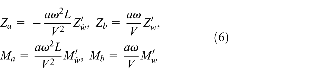
The viscous hydrodynamic coefficients derived from a direct resistance test and an oblique towing test were obtained by CFD and a hydrodynamic experiment. The results and errors are shown in Table 1.

Table 1.

Viscous hydrodynamic coefficients obtained by CFD and experiment.

Coefficients	$X'_{uu}$	$Y'_{vv}$	$Z'_{ww}$	$Y'_{v}$	$Y'_{v \| v \|}$	$Z'_{w}$	$Z'_{w \| w \|}$
CFD	−0.2626	−0.0037	−0.0151	−0.0001	−0.0202	0.0001	0.0009
Experiment	−0.3512	−0.0042	−0.0192	−1.23e−4	−0.0241	1.15e−4	9.45e−4
Error (%)	25.23	11.9	21.35	18.7	16.18	13.04	4.67

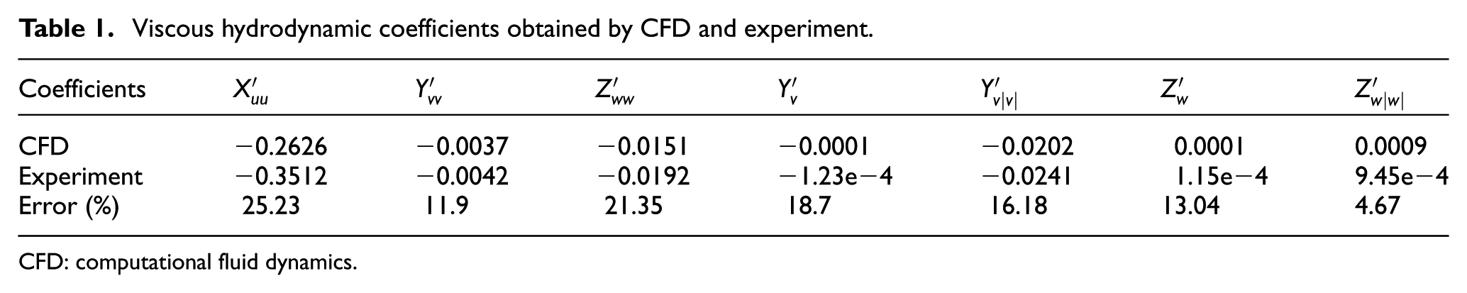
CFD: computational fluid dynamics.

To determine inertia hydrodynamic coefficients, a sinusoidal motion mechanism was designed similar to the planar motion mechanism: the mechanism was installed on the connection rod to generate sinusoidal motion of the model, as shown in Figure 8. The length of the oscillation rod was 0.6 m, the maximum frequency of oscillation was 1 Hz, and the maximum amplitude was 0.04 m.

Figure 8.

Diagram of planar motion experiment mechanism.

The frequencies measured were f = 0.2, 0.25, 0.3125, 0.4, 0.5, and 0.625 Hz; for the hydrodynamic coefficients related to pure heave motion, the hydrodynamic force Z and hydrodynamic moment M were measured at different frequencies by the six-component force sensor, and then, the coefficients were solved based on formulas (4)–(6). For the hydrodynamic coefficients related to pure sway, pure yaw and pure pitch motion can be obtained according to the algorithm similar to that introduced. Comparisons of the results of hydrodynamic coefficients by CFD and experiment are shown in Table 2.

Table 2.

Inertial hydrodynamic coefficients obtained by CFD and experiment.

Coefficients	$X'_{\overset{\cdot}{u}}$	$Y'_{\overset{\cdot}{v}}$	$N'_{\overset{\cdot}{v}}$	$Y'_{\overset{\cdot}{r}}$	$N'_{\overset{\cdot}{r}}$	$Z'_{\overset{\cdot}{w}}$	$M'_{\overset{\cdot}{w}}$	$Z'_{\overset{\cdot}{q}}$	$M'_{\overset{\cdot}{q}}$
CFD	−0.9747	−0.0949	−0.2226	−0.2226	0.0098	−0.8919	−0.215	−0.215	0.0138
Experiment	−1.092	−0.108	−0.2768	−0.1812	0.0072	−1.115	−0.2514	−0.2011	0.0102
Error (%)	10.74	12.22	19.58	22.85	36.11	20	14.47	6.91	35.29

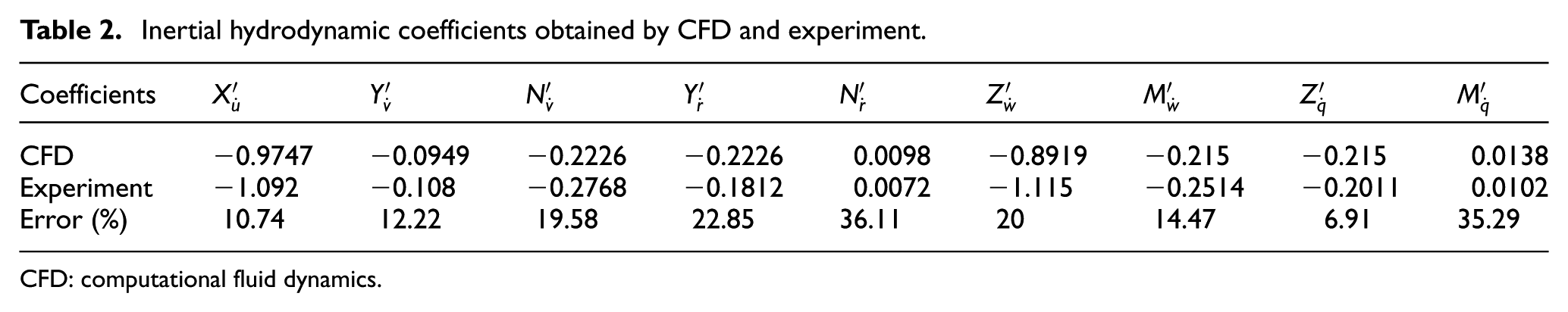
CFD: computational fluid dynamics.

To measure the wall hydrodynamic force, the robot was placed near the wall of the circular water tank. The wall distances were, respectively, set as l_w = 0.05, 0.1, 0.15, 0.175, 0.2, 0.25, 0.3, 0.35, 0.4, 0.45, and 0.5 m. Under the rated wall distance, the flow velocities were set at u = 0.1, 0.2, 0.3, and 0.4 m/s. The wall lateral and yaw hydrodynamic forces were obtained from the Y -axis and N -axis sensor data. By the same method, the wall hydrodynamic forces were measured for difference distances as shown in Figures 9 and 10.

Figure 9.

Force results of wall hydrodynamic force test: (a) flow velocity u = 0.1 m/s, (b) flow velocity u = 0.2 m/s, (c) flow velocity u = 0.3 m/s, and (d) flow velocity u = 0.4 m/s.

Figure 10.

Moment results of wall hydrodynamic force test: (a) flow velocity u = 0.1 m/s, (b) flow velocity u = 0.2 m/s, (c) flow velocity u = 0.3 m/s, and (d) flow velocity u = 0.4 m/s.

In Figure 9, the lateral hydrodynamic force Y increases slightly when the wall distance moves from 0 to 0.1 m and then has an obviously decreasing trend. By CFD, we find that the maximum lateral forces are, respectively, 1.41, 5.46, 9.94, and 13.85 N for u = 0.1, 0.2, 0.3 and 0.4 m/s. Several functions of the lateral hydrodynamic force and wall distance were obtained by MATLAB. A fitting function showed that the scopes of wall influence distance in the horizontal plane are, respectively, 0.44, 0.455, 0.472 and 0.485 m. In Figure 10, for the yaw moment of the wall effects, the trend is that the closer the wall, the smaller the results, and the CFD influence scopes are 0.85, 0.87, 0.895, and 0.915 m. From Figures 9 and 10, we conclude that there is some error between the CFD results and experimental results in the wall hydrodynamic test, but the error is acceptable, demonstrating the authenticity and reliability of simulation by CFD.

Conclusion

In this article, a semi-autonomous underwater robot was developed capable of welding the wall of a nuclear power pool in an emergency. To control the robot motion precisely, a hydrodynamic model was established, including hydrodynamic coefficients and a wall effect. Hydrodynamic coefficients in the theoretical model were found by developing a virtual hydrodynamic simulation test in CFD. The wall hydrodynamic force in the model was then quantified by CFD, and the influence scopes were, respectively, determined at different velocities by fitting functions. Finally, a prototype test was conducted in a circular water tank with and without the wall effect. The simulation results demonstrated that the wall hydrodynamic force, which was related to the wall distance and the robot velocity, was a main component of the model. By comparing the simulations with experimental results, the accuracy and authenticity of the simulation were verified, and the hydrodynamic model introduced was shown to be reasonable. In the near future, the wall hydrodynamic force will be calculated with the change in the wall distance when the robot moves vertically to the wall and a three-dimensional influent region of the wall on the robot can be obtained.

Footnotes

Handling Editor: Yangmin Li

Declaration of conflicting interests

The author(s) declared no potential conflicts of interest with respect to the research, authorship, and/or publication of this article.

Funding

The author(s) disclosed receipt of the following financial support for the research, authorship, and/or publication of this article: This work was support by the National Basic Research Program of China (2013CB035502). Special fund is National Natural Science foundation of China (61673138).

References

Guntzburger

Pauchant

. Complexity and ethical crisis management: a systemic analysis of the Fukushima Daiichi nuclear disaster. J Organ Eff 2014; 1: 378–401.

Matsushima

Ihara

Takase

et al . Assessment of radiocesium contamination in frogs 18 months after the Fukushima Daiichi nuclear disaster. Sci Rep 2015; 5: 9712.

Tadokoro

. Rescue robots and Fukushima-Daiichi nuclear power plant accident. J Robot Soc Jpn 2012; 30: 1017–1021.

Dong

Wang

Xing

et al . Design and control of a tracked robot for search and rescue in nuclear power plant. In: International conference on advanced robotics and mechatronics, Macau, China, 18–20 August 2016, pp.330–335. New York: IEEE.

Han

. Hydrodynamic forces and moments acting on a remotely operate vehicle with an asymmetric shape moving in a vertical plane. Eur J Mech B-Fluid 2015; 54: 1–9.

Cohen

Metzner

. Wall effects in laminar flow of fluids through packed beds. AICHE J 1981; 27: 705–715.

Eidsvik

. Identification of hydrodynamic parameters for remotely operated vehicles. Master’s Thesis, Norwegian University of Science and Technology, Trondheim, Norway, 2015.

Ridao

Tiano

El-Fakdi

et al . On the identification of non-linear models of unmanned underwater vehicles. Control Eng Pract 2004; 12: 1483–1499.

Obreja

Nabergoj

Crudu

et al . Identification of hydrodynamic coefficients for manoeuvring simulation model of a fishing vessel. Ocean Eng 2010; 37: 678–687.

10.

Avila

Nishimoto

Sampaio

et al . Experimental investigation of the hydrodynamic coefficients of a remotely operated vehicle using a planar motion mechanism. J Offshore Mech Arct 2012; 134: 46–51.

11.

Fan

Lian

Ren

et al . Loxodromic towing test at low speed and large drift angle for deep sea open-framed remotely operated vehicle. In: 2012 Oceans–Yeosu, Yeosu, South Korea, 21–24 May 2012, pp.1–5. New York: IEEE.

12.

Xie

et al . Hydrodynamic coefficients identification and experimental investigation for an underwater vehicle. Sens Transducers 2014; 164: 288–294.

13.

Nouri

Mostafapour

Bahadori

. An apparatus to estimate the hydrodynamic coefficients of autonomous underwater vehicles using water tunnel testing. Rev Sci Instrum 2016; 87: 065106.

14.

Jeong

Han

et al . Prediction of hydrodynamic coefficients for underwater vehicle using rotating arm test. J Ocean Eng Technol 2016; 30: 25–31.

15.

Petit

Paulo

Carlucho

et al . Prediction of the hydrodynamic coefficients of an autonomous underwater vehicle. In: IEEE/OES South American international symposium on oceanic engineering, Buenos Aires, Argentina, 15–17 June 2017, pp.1–6. New York: IEEE.

16.

Shojaeefard

Khorampanahi

Mirzaei

. Numerical investigation of oscillation frequency and amplitude effects on the hydrodynamic coefficients of a body with NACA0012 hydrofoil section. J Mech Sci Technol 2017; 31: 2251–2260.

17.

Anderson

. Computational fluid dynamics: the basics with applications. New York, NY: McGraw-Hill Press, 1995.

18.

Tyagi

Sen

. Calculation of transverse hydrodynamic coefficients using computational fluid dynamic approach. Ocean Eng 2006; 33: 798–809.

19.

Cheng

Lau

. Modeling and testing of hydrodynamic damping model for a complex-shaped remotely-operated vehicle for control. J Mar Sci Appl 2012; 11: 150–163.

20.

Wang

Huang

et al . An effective CFD approach for marine-vehicle maneuvering simulation based on the hybrid reference frames method. Ocean Eng 2015; 109: 83–92.

21.

Eng

Cheng

Lau

. Added mass computation for control of an open frame remotely-operated vehicle: application using WAMIT and MATLAB. J Mar Sci Technol 2014; 22: 405–416.

22.

Zhang

Cai

. Using CFD software to calculate hydrodynamic coefficients. J Mar Sci Appl 2010; 9: 149–155.

23.

Eng

Lau

Low

et al . Estimation of the hydrodynamic coefficients of an ROV using free decay pendulum motion. Eng Lett 2008; 16: 326–331.

24.

Pan

Zhang

Zhou

. Numerical prediction of submarine hydrodynamic coefficients using CFD simulation. J Hydrodyn 2012; 24: 840–847.

25.

Tang

Ura

Nakatani

et al . Estimation of the hydrodynamic coefficients of the complex-shaped autonomous underwater vehicle TUNA-SAND. J Mar Sci Technol 2009; 14: 373–386.

26.

Wang

Hao

et al . Analysis of hydrodynamic characteristics of unmanned underwater vehicle moving close to the sea bottom. Def Technol 2014; 10: 76–81.

27.

Suzuki

Inoue

Shimamura

et al . Experimental research on horizontal rotation of ROV induced by external forces near sea surface. In: Oceans 2008, Quebec City, Canada, 15–18 September 2008, pp.1–6. New York: IEEE.

28.

Zhu

Ying

Zheng

et al . Resistance test method on underwater vessel operating close to the bottom or the surface. J Ship Mech 2012; 16: 368–374.

29.

Zou

Larsson

. Computational fluid dynamics (CFD) prediction of bank effects including verification and validation. J Mar Sci Technol 2013; 18: 310–323.

30.

Liu

Song

Liang

et al . Design and experiment of control system for underwater ocean engineering structure inspection and cleaning remotely operated vehicle. In: Hung

Yen

(eds.) Frontier computing: theory, technologies and applications. Singapore: Springer, 2016, pp.865–879.

31.

Miao

Pang

. Development of a low-cost remotely operated vehicle for ocean exploration. In: Oceans 2015-MTS/IEEE Washington oceans, Washington, DC, 19–22 October 2015, pp.1–7. New York: IEEE.

32.

Anwar

Mohsin

Iqbal

et al . Design and fabrication of an underwater remotely operated vehicle (single thruster configuration). In: International Bhurban conference on applied sciences and technology, Islamabad, Pakistan, 12–16 January 2016, pp.547–553. New York: IEEE.

33.

Lewandowski

. The dynamics of marine craft: maneuvering and sea keeping. Singapore: World Scientific, 2004.

34.

Kim

Choi

et al . Estimation of hydrodynamic coefficients for an AUV using nonlinear observers. IEEE J Oceanic Eng 2002; 27: 830–840.

35.

Fan

Lian

Ping

et al . Oblique towing test and maneuver simulation at low speed and large drift angle for deep sea open-framed remotely operated vehicle. J Hydrodyn 2012; 24: 280–286.

Hydrodynamic calculation and analysis of a complex-shaped underwater robot based on computational fluid dynamics and prototype test

Abstract

Keywords

Introduction

Structure and function of robot

Hydrodynamic model

Hydrodynamic coefficients solved by CFD

Unsteady motion simulation test

Steady-state motion simulation

Wall hydrodynamic force solved by CFD

Prototype test

Conclusion

Footnotes

Declaration of conflicting interests

Funding

References