Purified orbit diagram and numerical study for a failure analysis of a Sirocco fan

Abstract

Sirocco fan units are very common and widespread solution for air conditioning used in public transportation applications (buses or trains). The users’ comfort and tranquillity are main concerns in the automotive industry. Inside such turbomachines, the flow structure always becomes highly three dimensional and unsteady, compromising the referred comfort, and sets the focus on the working flow variables. A mathematically exact solution for that flow, which would provide any required information on pressure or forces, is out of scope at the current engineering design processes. Nevertheless, some flow features and mechanical data are needed to progress in the frame of a modern industrial environment, which each time more strongly, besides the different design procedures, involves maintenance protocols. The correctness of a given maintenance protocol relies on its feasibility to handle a set of machine working parameters or variables, including a number of them as wide as possible. Doing so, a set of non-dangerous ranges for them can be established. Such ranges are often defined promoting a series of failures similar to real ones, when the machine is in its usable lifetime. In what refers to the flow analysis, a reasonably good tool has been developed using a computational fluid dynamics technique and, from the experiments, a better understanding of the fan operating conditions is accomplished. For a Sirocco fan unit and to establish proper working ranges for maintenance purposes, a series of failures have been experimentally and numerically tested. Initially, real data from industry have been required and a list of main failures was made. It included impeller or rotor unbalance, impeller channel obstruction and blocked inlet. The first two failures are studied using a purified orbit diagram technique and the last one is numerically analysed. All four working conditions are studied for at least three different flow rates and, therefore, a deeper insight into the fan working parameters and options is made feasible. In the frame of the maintenance protocol, a full set of ranges for the considered failures have been obtained.

Introduction

Squirrel or Sirocco fans are forward-curved blade centrifugal turbomachines. Very often, they are manufactured in small sizes and commonly used in public transportation. Other practical applications cover a wide range of industrial plant usages and they are also widespread in transportation applications (buses, trains and so on). The name Sirocco fan was introduced by the classic textbook by Eck, ¹ where a global frame of the existing geometries is given. More recently, Rouse ² has commented on the global variables of these units, in the frame of a general fan classification. Their relative small dimensions and low cost make them competitive for residence heating systems, automotive units or other industrial applications. Their working parameters include a high specific speed and a large width-to-diameter ratio (b/D₂), while the flow deceleration imposed by the diameter increase precludes the separation inception, as explained by Kind. ³ Other important features, such as the short chord and the large number of blades, were previously pointed out by Kind and Tobin, ⁴ where a particular and detailed study of the geometry and flow implications is given. Globally speaking, these kinds of units become an economic solution when dealing with a small unit for a relatively high flow rate delivery.

Due to the above mentioned interest and current applications, the number of classical studies on forward-curved centrifugal fans is quite large and ranges from the initial experimental search for secondary flow patterns ⁵ to more advanced and complementary experimental and numerical works. ⁶ Other and more recent studies, for instance, Kim and Seo, ⁷ Engin ⁸ and Velarde-Suárez et al.,^9,10 have proposed a series of geometrical modifications or rearrangements to improve some given design parameters such as, the performance enhancement or the noise reduction, among others. Particularly, Engin ⁸ studied the flow in the tip region of centrifugal fans, using a numerical approach. In the same frame, and as a starting point for the work presented here, the study by Ballesteros-Tajadura et al. ¹¹ has shown a numerical solution for the pressure fluctuations in the volute of a centrifugal fan unit.

The importance of a proper definition of a maintenance protocol for any kind of mechanical machine is deeply referred in the bibliography and several works are available; for a wide review on the topic, refer to Jardine et al. ¹² The particular features for rotating machines and different approaches are explained in Chen et al., ¹³ Shi ¹⁴ and Cui and Craighead. ¹⁵ Regarding failures diagnosing fans, a number of very important frequencies are numbered in Chen et al. ¹³ as theoretical values. Failure characteristics or diagnostic indexes cannot be defined quantitatively, but other failure characteristics are clearly observed, as explained in Shi. ¹⁴ On the other hand, the fast Fourier transform (FFT) has been established as standard method to obtain the corresponding spectra revealing its composition in the frequency domain; see examples in Shi ¹⁴ and Shi et al. ¹⁶ Nevertheless, some other methods are available in the literature, see, for instance, Shibata et al. ¹⁷ and Sheard et al., ¹⁸ and may also be considered as relevant tools.

Similar to what is targeted in this article, combining both methodologies (numerical and experimental), a study about the flow in a forward-curved centrifugal fan was proposed by Lin and Huang. ⁶ Focusing on the thermal performance of small units used for cooling purposes in personal computers (PCs), they provide a quite ambitious parametric study of the aerodynamic and sound properties of different geometries, both experimentally and numerically. And, in a more recent date, the work by Montazerin et al. ¹⁹ calls again the attention on the inlet flow performance of these units, previously suggested by Kind. ³

Considering the previously mentioned studies and many other important contributions which might be found in the bibliography, the interest on the topic is clear. This work takes into account the researchers’ concern about the definition of a maintenance protocol using an experimental approach. A purified orbit diagram (POD) technique is used to complement previous efforts of the research group, according to different previous publications.^{9,10,11,20–23} It can be considered in the frame of previous works by the same working team, see, for instance, Velarde-Suárez et al., ⁹ Ballesteros-Tajadura et al.,^11,20 González et al. ²¹ and Delgado et al.^22,23

Experimental set-up and measurements

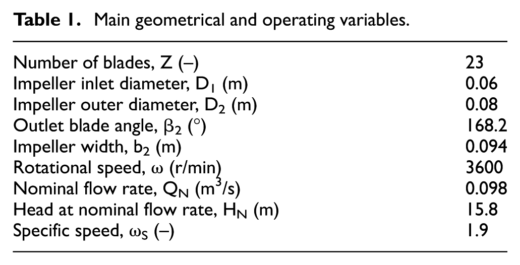
For the particular application, a squirrel cage fan unit to be studied is built with a pair of twin impellers’ unit, arranged as shown in Figure 1 (left sketch). The two impellers are placed on both sides of the electrical motor and supported by the two sides of the shaft in cantilever, from its central position. The shaft also produces the rotation of both impellers in a forward direction and, for each one, a staggered configuration with a middle plate that splits up the impeller into two parts: the motor side and the free inlet side. The staggering of the two parts means that they are mounted producing a shift of the 23 blades, so that the mechanical resonances are minimized. Therefore, in such arrangement, there is a free inlet, at each impeller side opposite to the placement of the motor. And there is also an obstructed inlet, on the motor side of each impeller. From the manufacturing point of view, each impeller is built with two parts, which are linked together by a central plate, as can be observed in Figure 1 (left sketch). The total width of the whole impeller is 0.094 m. Covering the whole unit, there is a volute or external casing, providing two rectangular outlet sections. Complementary main geometrical variables are shown in Table 1. The main working parameters at the nominal conditions are also shown in Table 1.

Figure 1.

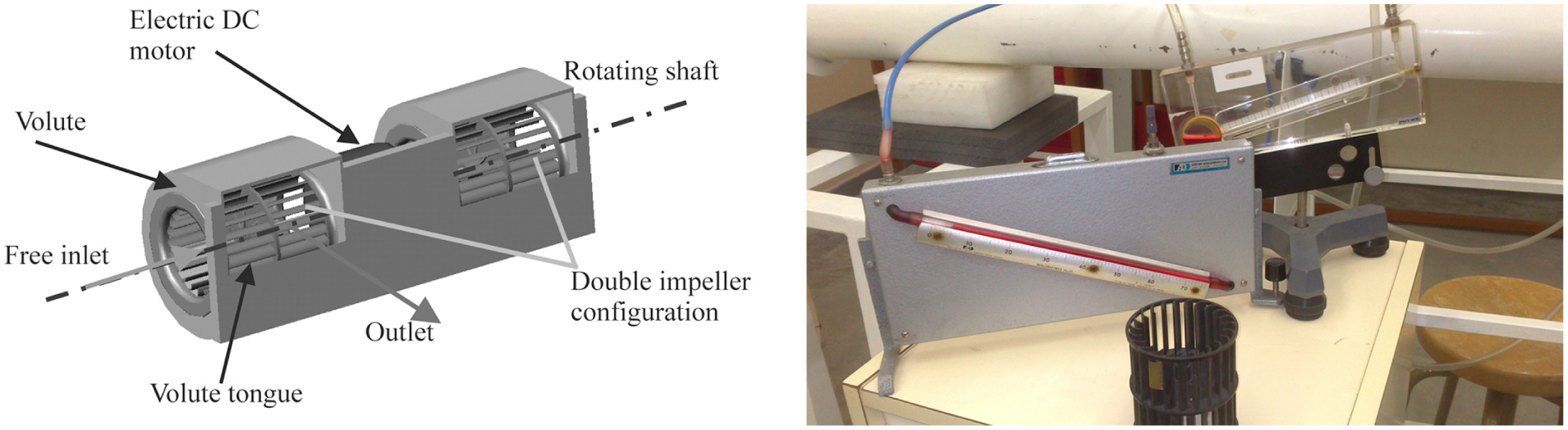
Simplified sketch of the tested fan (left) indicating the most important features and both static and differential manometers (right), with one impeller in the foreground.

Table 1.

Main geometrical and operating variables.

Number of blades, Z (–)	23
Impeller inlet diameter, D1 (m)	0.06
Impeller outer diameter, D2 (m)	0.08
Outlet blade angle, β2 (°)	168.2
Impeller width, b2 (m)	0.094
Rotational speed, ω (r/min)	3600
Nominal flow rate, QN (m3/s)	0.098
Head at nominal flow rate, HN (m)	15.8
Specific speed, ωS (–)	1.9

The geometrical and working parameters of the fan can be found in more detail in a previous work by the group; see Ballesteros-Tajadura et al. ²⁰ To determine the performance curves, the basic procedures are performed following ISO 5801:2007, which splits the calculation of the flow rate and head into two different procedures. The flow rate has been obtained using a Pitot tube, connected to a differential manometer (see Figure 1, right). First, a calibration of the pipe for a known flow rate is performed promoting a series of traverses to get the velocity profile at different radial positions and the maximum pressure difference or maximum flow velocity, which is retrieved at the middle or centre point of the pipe. Then, a relationship or calibration chart is built up for the flow rate as a function of the centre point dynamic pressure. With such calibration chart, for a given measurement of the dynamic pressure (with the Pitot and the differential manometer), the unknown flow rate is then obtained. For the stagnation pressure or total head, the sum of three main terms was considered (static, dynamic and friction losses). The static pressure is measured with standard pressure taps connected to a manometer (see Figure 1, right), using an average from four different angular positions, as stated in the Standard. The dynamic pressure comes from the Pitot tube measurements, also corrected following the Standard indications. And, finally, the losses are obtained by extrapolating the equivalent ones which are measured from a known length between two different static pressure locations. A final correction for the dynamic pressure is introduced, according to the Standard.

As it will be explained in what follows, this procedure was repeated for a total of 18 different working points, both in the baseline and for the tested failure, to obtain the performance curves. Nevertheless, for most part of the study, only the reference maximum pressure in the centre of the pipe becomes important to be able to compare different working conditions. Finally, repeatability tests were carried out for the different measurements, and after correction for the air density the uncertainty for the flow rate is found to be less than 5% in all measuring points and for most points is found to be below 2.1%. The head uncertainty was always below 1.5%.

To consider a given fault diagnosis protocol, different measurements must be taken for different operation conditions producing, in such way, different standard faults for the fan under study. The obtained measurements will provide a possible comparison of the observed change in the fans’ performance with the baseline, or operation without any fault. In this study, apart from the baseline operation, two different faults have been considered for the experimental study: one blade-to-blade channel obstruction and an unbalanced impeller operation. Finally, an inlet blockage has been numerically analysed. The facility, properly instrumented to carry out the designed measurements, was arranged as shown in Figure 2. The fan is placed on one end of the pipe, and in the other end, a regulation cone is installed. As complementary noise measurements have also been carried out, placement of the microphones is shown, although they were not used for this study. Here, the studied variable is the vibrating state of the fan. For such state to be defined, two B&K-4384 fast response piezoelectric accelerometers are available. They are connected to a charge amplifier, B&K-2635, especially suitable for acceleration measurements. The sensitivity of the sensors is 10 pC/g. The cut frequency for the accelerometers is 10 kHz, although, and due to the arrangement, the maximum valid frequency is found to be 3 kHz. The measurements’ chain is completed with the acquisition unit Harmonie, connected to the PC. The whole set-up is schematically represented in Figure 3. Repeatability tests were carried out for several configurations and flow rates and have shown maximum value with variation in characteristic peaks below 3%. To account for the fan working point, three different flow rates were studied: nominal one and two off-design working points (one at 0.7 and other at 1.3, respectively, and relative to the nominal one).

Figure 2.

Available fan installation for the experimental measurements.

Figure 3.

Measurements’ chain sketch.

After the signal was recorded for a set of three working points and three operation conditions, the signal analysis was then handled, as is explained in what follows.

POD technique for the baseline and two failures

The POD technique consists of a spectral analysis technique that may be applied to different measurements when those evolve within a time framework. In the particular application studied in this article, a POD technique is applied to the horizontal and vertical signals recorded from the two sensors used (see Figure 4 for the global setting of the sensors at the fan casing).

Figure 4.

Accelerometers’ positioning during the experiments.

An example of the time signal recorded is shown in Figure 5 for nominal flow rate and baseline operation. These kinds of signals were recorded for the three different operations and for three representative flow rates.

Figure 5.

A given time signal recorded for the baseline operation.

The implemented procedure, following Chen et al., ¹³ works as follows:

1. Measurement of the time signal for the horizontal and vertical components of the acceleration. The acceleration is recorded as a function of the time, following the experimental routine and apparatus previously described.

2. Apply a standard FFT to get the frequency decomposition of the signals. The information is transformed into a set of data (f_k, ϕ (k)), that is, into the frequency domain, and the energy components are split for the different frequencies.

3. Search for the predominant frequencies with their relative values and obtain the (so called) modified spectrum of the signal (S). This new value is a simplification of the real spectrum considering only N frequencies of interest or relatively more intense than the others. Therefore, S is a filtered spectrum at the stronger measured frequencies. In our particular application, the following are found to be the most relevant frequencies (not all affect all operations, but no others related to electrical or others were found to be important), as shown in Table 2.

4. Apply the POD technique to get the purified spectrum. The following equations are considered to obtain the horizontal and vertical components of the orbit diagram

$$\{\begin{array}{c}({\mathrm{X}}_{\mathrm{x}}{)}_{\mathrm{j},\mathrm{POD}}=\sum _{\mathrm{k}=1}^{\mathrm{N}}{\mathrm{S}}_{\mathrm{x}}(\mathrm{k})\cos (2\mathrm{\pi }\mathrm{j}{\mathrm{f}}_{\mathrm{k}}+{\mathrm{\varphi }}_{\mathrm{h}}(\mathrm{k}))\hfill \\ \multicolumn{1}{c}{({\mathrm{X}}_{\mathrm{y}}{)}_{\mathrm{j},\mathrm{POD}}=\sum _{\mathrm{k}=1}^{\mathrm{N}}{\mathrm{S}}_{\mathrm{y}}(\mathrm{k})\sin (2\mathrm{\pi }\mathrm{j}{\mathrm{f}}_{\mathrm{k}}+{\mathrm{\varphi }}_{\mathrm{v}}(\mathrm{k}))}\end{array}$$

(1)

Table 2.

Main frequencies considered for the POD analysis.

f	Mechanical meaning
1	Rotational frequency
2	Second harmonic of the rotational frequency
3	Third harmonic of the rotational frequency
4	Fourth harmonic of the rotational frequency
8	Eighth harmonic of the rotational frequency
16	Sixteenth harmonic of the rotational frequency

The full orbit diagram would be the result of plotting equation (1) for the whole set of valid and selected frequencies, within the limits of the experimental measurements’ chain, disregarding the ones with lower amplitude. In the performed measurements, the upper limit for the frequencies goes to 3 kHz; the orbit sums in equation (1) point to a number N quite high. Nevertheless, and once the experiments were carried out, the N value becomes much lower. Particularly, in this article, N is a value less than 5 in all the studied conditions.

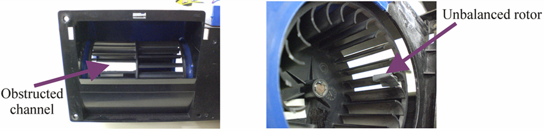
Therefore, the purified spectrum depends only on a few values, but stronger or more relevant frequencies. If there is a change in value or phase for any other frequency, the spectrum will remain constant. First, the nominal flow rate is considered, and then two others were analysed, a low and high one, respectively, to cover the possible fan working range. The three operation conditions considered at the experimental campaign were the normal one (baseline operation), the obstructed channel and the unbalanced shaft operation. The impeller arrangement for these failures is shown in Figure 6. A detail of the obstructed channel failure is shown in Figure 6 (left figure). For the unbalance of the shaft, small metal pieces of 1.6 g (including the fixing material) were fixed up to one of the fan blades, as can be observed in Figure 6 (right figure). Although a third failure was studied, namely, a blockage of the inlet duct (already explained in Delgado et al. ²² ), the results for this case are only numerically analysed, as will be explained.

Figure 6.

Comparison of performance curves.

An example of the measurements after application of the FFT procedure is shown in Figure 7. It corresponds to a low flow rate and the baseline operation. As can be read in Chen et al., ¹³ the expected peaks and their meaning are always quite clear for rotating machinery. From most relevant peaks, a set of failure conditions might be analysed. Nevertheless, the focus of this article is to find out the most relevant frequencies to achieve or define a good diagnosis for the studied failures. With this purpose in mind, a full study of the relevant peaks is mandatory and the result would be analysed in detail in what follows.

Figure 7.

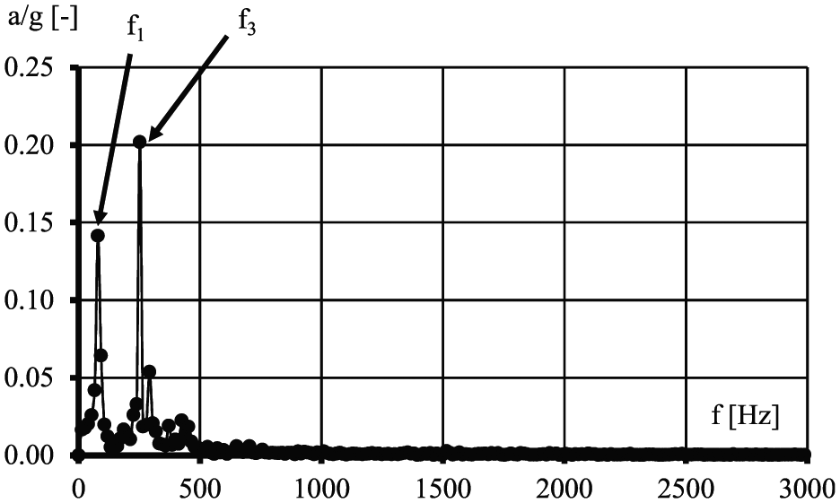
Typical values by applying the FFT to the obtained measurements.

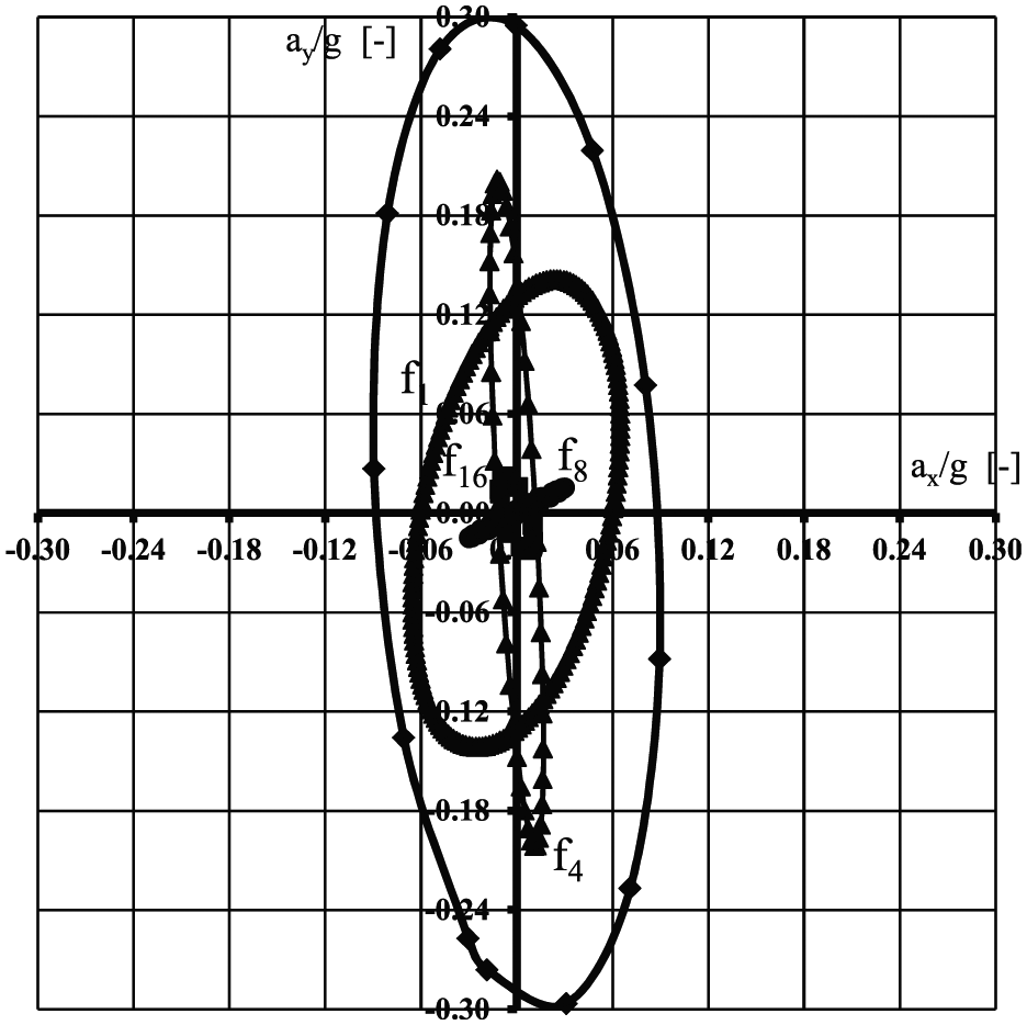
From the kind of spectrum as the one shown in Figure 7, the POD technique is then applied to the nine studied data sets, namely, the three flow rates and three different operating conditions. After peak selection, Figure 8 shows the composition of peaks and the resulting diagram for the nominal flow and the normal (baseline operation). As the resulting diagram is a summation of vectors, the result is obtained as such for the first point. Doing this for a full rotation of the blades (a 360° turning of the impeller), the result is the plotted diagram; see the outer or envelope curve in Figure 8. In this particular graph, the result is the summation of the three most relevant frequencies: f₁, f₂ and f₄. Also, the strongest signal or the most relevant one is the rotation frequency (f₁). Then, the fourth harmonic can be appreciated as the second stronger one and, finally, the second harmonic with relatively less importance. Other harmonics influence even in a lower level and, therefore, are not considered, obtaining in such way the POD of the signal. The vector summation of the three components is the result shown in Figure 8 (only the first point of the data set is remarked) and it resembles the POD graph of the nominal flow rate at the baseline operation of the fan. It shows a maximum vibration resultant for an angle near 45°, which indicates the almost equal contribution of the vertical and horizontal components in the vibration of the machine. For each rotation of the impeller, the composition of the x and y components, for a given flow rate, completes one of the elliptical-shaped figures (similar to the one in Figure 8).

Figure 8.

Vector summation of the different frequencies for the nominal flow rate.

The procedure is then repeated for the low and high flow rates. The result for the high flow rate and baseline operation is shown in Figure 9. The predominant frequencies are, for this working point, the rotating and the four basic harmonics. Again, the vector summation is showed for the first point. The POD graph for this flow rate becomes more vertical than the one obtained in Figure 8. In this flow rate and operating at the baseline condition, the vertical component of the force is more important than the horizontal one. The equivalent result for the low flow rate is shown in Figure 10. The most important frequencies are, for this condition, the rotating one and the 4th, the 8th and the 16th harmonics. As for the high flow rate, the vertical component becomes predominant and the POD is almost vertical, with a relation 3:1 of the maximum vibration levels, that is, the vertical maximum being three times the horizontal one. Therefore, off-design flow rates give rise to predominantly vertical vibrations.

Figure 9.

Vector summation for the high flow rate.

Figure 10.

Vector summation for the low flow rate.

Note that the scale for Figures 8–10 is not the same and, therefore considering this scale change, the relative importance of each POD is re-scaled and compared in Figure 11. The comparison shows the less important vibration at a high flow rate, although of an order of magnitude quite close to the nominal flow rate one. The highest vibrating levels are found for the low flow rate, with maximum vibration almost twice as the maximum for the other two analysed flow rates.

Figure 11.

POD for the three studied flow rates and baseline operation.

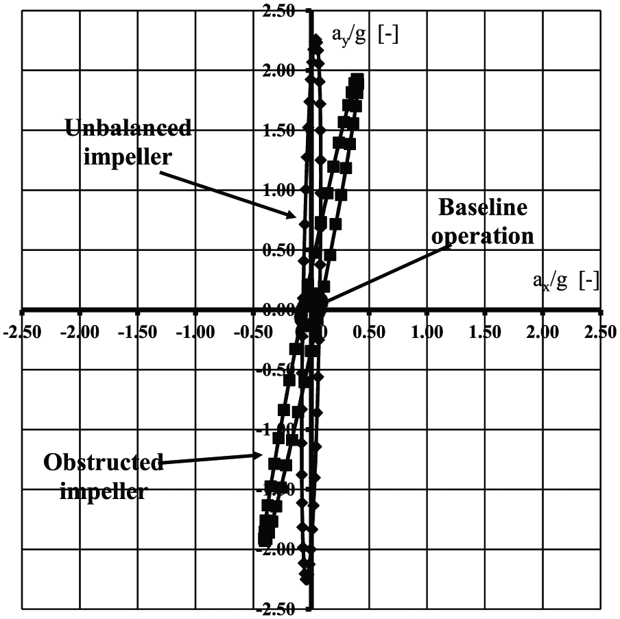
Similar comparison is possible for the unbalanced rotor and the obstructed channel operations. Figure 12 provides the comparison as a function of the flow rate for the unbalanced rotor operating condition. The final comparisons, and more relevant in terms of fan operation and fault diagnosis, are the graphs showing the results for the same flow rate and different operation conditions. Such graphs are plotted in Figures 13–15. The scale is fixed for the nine studied data sets, to allow comparison among them.

Figure 12.

Comparison of the POD for the three flow rates: unbalanced rotor operating condition.

Figure 13.

POD comparison for the nominal flow rate.

Figure 14.

POD comparison for the low flow rate.

Figure 15.

POD comparison for the high flow rate.

In particular, Figure 13 shows the comparison of the POD for the nominal flow rate. A minimum vibrating value is found for the baseline configuration, and a similar behaviour is found for both the studied failures. In fact, the baseline operation shows vibration levels in the order of six times lower than the failure ones. The impeller unbalance gives rise to the highest vibrations, with a maximum of nearly 2.5 times the gravitational acceleration. The main component for the three configurations is almost vertical, meaning that this is the main stress direction for such operation.

In Figure 14, the POD for the low flow rate is plotted. Again, the lower vibrations are found for the baseline configuration. The higher vibrations are found for the unbalanced impeller when this operating condition is compared with the baseline operation. In this flow rate, there is even a higher ratio of difference when comparing the baseline operation with the unbalanced impeller failure (around 10 times lower). The obstructed impeller vibrations show an almost circular shape, not as elliptic as in the other flow rates and, therefore, both vertical and horizontal maximum are of the same order or magnitude. The vibrations for the baseline operation are one third of the ones for this failure. The maximum acceleration found is around 2.5 the gravity one and the main direction is the vertical one.

Figure 15 plots the POD for the highest analysed flow rate. According to the previous results and to what it might be expected, the minimum is found for the baseline operation. The relative values are around 20 times lower than the ones for the unbalanced rotor. The obstructed channel operation shows a medium range of vibrations, around 12 times higher than the baseline operation values. For off-design flow rates, the unbalanced impeller fault results in even higher accelerations, while for the nominal flow operation, both studied faults produce equivalent acceleration levels. The maximum acceleration for this flow rate is around 1.5 times the gravitational one, and the main direction is again the vertical one. The ratio between the maximum acceleration for a given failure and the baseline operation becomes the order of up to 20 times.

As a conclusion, the POD results allow a clear distinction between the baseline and the fault operations; however, the difference between the two failures tested is not clear. The neatest way to recognize the kind of failure from the experiments would be the angle of the main vibration, which is always more vertical for the unbalanced impeller operation. The maximum vibrations are found for the vertical direction, and the ratio between the different failures and the baseline ranges from 3 to 20 times, the maximum acceleration being around 2.5 times the gravitational one.

Numerical model

There are many other possible failures that cannot be easily compared to the previous ones, because they could affect the flow rate and, therefore, the working point of the studied fan. This is what happens when considering the inlet section blockage that may appear in practice when some piece of matter is stuck in the inlet section by action of slight pressure that affects the air income at that section of the fan. To handle the mentioned failure, a numerical study is proposed to obtain the comparison between it and the baseline operation.

Then, to handle the more advanced problem of considering the inlet blockage section, a three-dimensional (3D) geometrical model was developed for the whole machine. The flow in this geometrical model has been solved using the commercial code FLUENT^® which, by a finite volume algorithm, solves the unsteady Navier–Stokes equations for an unstructured mesh, allowing the impeller relative motion. Such commercial codes have shown their feasibility in handling turbulent and unsteady flow features in the past decades and, particularly, in the turbomachinery field. A SIMPLEC algorithm is chosen for the pressure and velocity coupling, while second-order, upwind discretizations have been used for convection terms and central difference schemes for diffusion terms. The continuity and momentum equations for a 3D flow are

$$\frac{\partial \overrightarrow{\mathrm{G}}}{\partial \mathrm{t}}+\nabla \overrightarrow{\mathrm{F}}=\overrightarrow{\mathrm{S}}$$

(2)

where $\overrightarrow{\mathrm{G}}$ is the vector of conservation variables, $\overrightarrow{\mathrm{F}}$ is the flow vector and $\overrightarrow{\mathrm{S}}$ is the source terms’ vector, namely

$$\overrightarrow{\mathrm{G}}=\left[\begin{array}{c}\mathrm{\rho }\hfill \\ \multicolumn{1}{c}{\mathrm{\rho }{\mathrm{U}}_1}\\ \multicolumn{1}{c}{\mathrm{\rho }{\mathrm{U}}_2}\\ \multicolumn{1}{c}{\mathrm{\rho }{\mathrm{U}}_3}\end{array}\right],\overrightarrow{\mathrm{F}}=\underset{\mathrm{j}=1,2,3}{\left[\begin{array}{c}\mathrm{\rho }{\mathrm{U}}_{\mathrm{j}}\hfill \\ \multicolumn{1}{c}{\mathrm{\rho }{\mathrm{U}}_1{\mathrm{U}}_{\mathrm{j}}+\mathrm{p}\overrightarrow{\mathrm{i}}-{\mathrm{\tau }}_{1\mathrm{j}}}\\ \multicolumn{1}{c}{\mathrm{\rho }{\mathrm{U}}_2{\mathrm{U}}_{\mathrm{j}}+\mathrm{p}\overrightarrow{\mathrm{j}}-{\mathrm{\tau }}_{2\mathrm{j}}}\\ \multicolumn{1}{c}{\mathrm{\rho }{\mathrm{U}}_3{\mathrm{U}}_{\mathrm{j}}+\mathrm{p}\overrightarrow{\mathrm{k}}-{\mathrm{\tau }}_{3\mathrm{j}}}\end{array}\right]},\overrightarrow{\mathrm{S}}=\left[\begin{array}{c}0\hfill \\ \multicolumn{1}{c}{{\mathrm{S}}_{{\mathrm{M}}_1}}\\ \multicolumn{1}{c}{{\mathrm{S}}_{{\mathrm{M}}_2}}\\ \multicolumn{1}{c}{{\mathrm{S}}_{{\mathrm{M}}_3}}\end{array}\right]$$

(3)

In equation (3), p is the static pressure, ρ is the fluid density, t is the time, ${\overline{\mathrm{U}}}_{\mathrm{j}}$ are the velocity components, ${\tau }_{\mathrm{ij}}=-\rho \overline{\mathrm{U}{\prime }_{\mathrm{i}}\mathrm{U}{\prime }_{\mathrm{j}}}$ is the viscous stress tensor and ${\mathrm{S}}_{{\mathrm{M}}_{\mathrm{j}}}$ , are the momentum source terms. More precisely, the viscous stress tensor ${\tau }_{\mathrm{ij}}$ , is afterwards related to the mean velocity gradients using the Boussinesq approach. In this study, a standard k–ε two-equation model to simulate the turbulence is used. This choice has shown its robustness and reliability when simulating centrifugal fans, capturing accurately enough a wide range of flow details near the tongue region and in the jet-wake pattern (see, for instance, Ballesteros-Tajadura et al., ¹¹ where a more detailed term split is explained).

A compatible pre-processor, GAMBIT v2.0, was used to develop both geometries and meshes. The discretization of the geometry was done keeping an optimal ratio between calculation time and the accuracy order of the simulation for the flow studied characteristics.

To account for the impeller relative rotation, a sliding mesh technique was implemented in the numerical model. Some numerical tests were carried out to assure the interface connection of the flow variables and the results were obtained to optimize the number of cell points in that area. Two interfaces were defined to apply the sliding mesh technique. A full domain discretization is performed using around 1 million prismatic cells. Unstructured cells have shown good behaviour to account for critical flow features as separation and were considered appropriate for the present application. Figure 16 shows a sketch of the final mesh on top of the figure. Only half of the machine is shown and some surfaces have been removed to properly observe the blades inside the machine. The final mesh defined for the studied geometry was obtained as a compromise between the grid dependence tests and the calculation time. Special care was taken in the definition of the flow channels between each blade, and a denser grid was defined in such zone. Also, the region near the volute tongue was considered critical and mesh refinement is also applied there. A sketch with the blocked inlet and different parts is shown in the bottom of the figure.

Figure 16.

Sketch of the final mesh for half of the machine, without (up) and with the blocked inlet (down).

Different mesh independence tests were carried out to observe that the evolution and errors in the solution due to the mesh were found to be kept under a very low value and always much lower to the experimental uncertainty, for an increasingly finer mesh, in comparison with the one finally used. The total pressure coefficient at the flow coefficient where the fan exhibits its best efficiency point was used to determine the influence of the mesh size on the solution. The convergence criterion was set to a maximum residual of 10⁻⁶. According to the referred preliminary tests, the grids with the highest number of mesh cells were considered to be sufficiently reliable to assure mesh independence. However, there are still some tests to be performed.

Flow model and numerical accuracy

For the unsteady calculations, the number of iterations for each time step has been adjusted to reduce the residual below an acceptable value. For all the fan working points and operating conditions, the ratio between the sum of the residuals and the sum of the fluxes for a given variable in all the cells is reduced to the value of 10⁻⁵ (five orders of magnitude). Initializing the unsteady calculation with the steady solution, more than 17 impeller revolutions (approximately 5000 time steps) were necessary to achieve the convergence of the periodic unsteady solution. The refined discretization, together with the small time step, chosen to catch the main unsteady phenomena, imposed quite critical and hardware demanding calculations, only affordable with a proper parallel computing protocol. More precisely, the code was run in a cluster of 16 Pentium 4 (2.4 GHz) nodes. The time step for the unsteady calculations was set to 7.25 × 10⁻⁵ s (equivalent to 10 time steps per blade passage, or 230 time steps per impeller revolution) to obtain a reasonable time resolution, capable to capture the main unsteady phenomena involved. More details on the numerical process have been published in previous works (see Ballesteros-Tajadura et al. ¹¹ ).

The numerical accuracy of both steady and unsteady results was estimated to be always below 1.5% and 0.5%, respectively. During the numerical study, the guidelines proposed by Freitas ²⁴ were used, and the numerical uncertainty was related to change in certain reference values when different mesh refinements were considered. A series of test to accomplish the more recent validation procedures, by Celik et al. ²⁵ and comments by Roache, ²⁶ were also considered, and similar conclusions on the numerical accuracy were obtained.

For a deeper insight on the model itself and steady flow comparisons (numerical versus experimental) and an extended inlet flow study, see Ballesteros-Tajadura et al. ¹¹ The impeller flow-averaged flow fields and the outlet flow velocities are considered as first approach here, to end with the outlet velocity field. All these are shown to find some possible correlation with the previously analysed experimental results. Particularly, for the global variables, head and flow rate, less than 0.3% change was reported using a mesh size of the order of half of the one finally chosen. For the local variables and the steady model, pressure and velocity, changes higher than 1.0% could be consider exceptional, again comparing the actual mesh and the one with a mesh size of the order of half of it. Very few differences could go up to 1.2%. The steady results were always giving slightly higher differential values than the unsteady calculation. The last ones were only checked with the two meshes for two flow rates, and there the differences were always below 0.5%.

Numerical results

As a first step in comparison, a performance curve analysis is carried out to obtain the model. Figure 17 shows clearly the effect of the proposed failure, with a dramatic shortening of the flow rate range or possible working points of the fan under study. The nominal or best efficiency point decreases in a factor of the order of 2, from $\phi$  ≈ 0.6 to $\phi$  ≈ 0.3. Such big change in working points makes an experimental comparison of two possible equivalent points non-effective, and it is the reason behind the numerical approach presented in this part. A quite good agreement is found for the comparison of the two set of curves, baseline and inlet blockage, obtained numerically and experimentally. However, a quite constant difference is found for the blockage operation condition when the comparison of numerical–experimental is observed. The difference looks as a static pressure offset, but the conditions of the measurements and numerical results were extensively checked to find out possible errors in what refers to it, and no clear conclusion could be drawn. On the other hand, the comparison for the baseline operation is really good and only slight differences are found at low flow rates. Probably, some separation conditions are not well captured by the numerical model and, probably, the turbulence model is over-estimating losses. Flow details are analysed in what follows.

Figure 17.

Performance curve comparisons for the baseline and blocked inlet failure.

Particularly, the blade-to-blade flow evolving in the impeller is quite relevant for a numerical study. In the following figures, the flow velocity in the impeller is studied. Two different axial sections are considered, one placed on free inlet half of the impeller and another on the obstructed inlet (motor side). At both sections, the relative velocity is plotted in a 0–22 m/s scale to allow comparison between different sides and different flow rates. Also, the free and motor side flow fields are considered. The blockage of the inlet promotes flow conditions intermediate between the free inlet and the total blockage and, therefore, the comparison is considered relevant here.

Figure 18 shows the relative velocity in the impeller for a low flow rate on the free inlet side of the impeller. The volute is depicted in the figure to place the volute tongue, and the selected plane for representation is mid span of the blades. A quite axi-symmetric pattern is found. This is found for all the circumferential positions, except for those placed after the volute tongue (in the impeller rotation direction, that is, in the clockwise direction in Figure 18). In the region after the volute tongue, a low-velocity or stagnation region is found for this low flow rate. On the other hand, for the rest of the impeller, a flow acceleration is found at the blades’ outlet section, pointing to a clear flow separation. On the other side of the impeller, that is, in the obstructed region, as shown in Figure 19, the flow relative velocity shows a similar behaviour. There is a global velocity decrease (less mass flow enters through this section), but again the flow is quite axi-symmetric, with a stagnation region in the after-tongue region. The velocity increase in the blades’ outlet section is not so strong.

Figure 18.

Averaged relative velocity for high flow rates ( $\phi$  = 0.766, contours for the free inlet side).

Figure 19.

Averaged relative velocity for high flow rates ( $\phi$  = 0.766, contours for the motor inlet side).

For the nominal flow rate and the free inlet impeller, almost the same trend is found, that is, almost axi-symmetric pattern, except in the angular region placed from 0° to 45° in the rotating direction and from the position of the volute tongue. In the mentioned region, there is a lack of velocity and the effect of the impeller exit separation is not so clear.

In the obstructed inlet impeller, there is less velocity than in the free inlet side. However, the flow differences in the angular direction are more evident, with a less symmetry as in the previous figures. The effect of the volute tongue is more important and, therefore, the flow stagnation produced is also clearer. A first difference, for the baseline operation, is shown in Figures 18 and 19, where the averaged velocity fields in the rotating frame for a high flow rate are plotted. Figure 18 corresponds to the free inlet impeller, while Figure 19 corresponds to the motor side inlet impeller. However, both figures look very similar, with half of the impeller opposite to the volute tongue showing a very axi-symmetric pattern. On the other hand, the two other quarters of the impeller, as they would be divided by a fictitious line traced from the centre of rotation to the volute tongue, show quite different behaviour. In the upper quarter, there is a high-velocity region. In the lower one, there is a low velocity zone, equivalent to the one found in the previously analysed flow rates.

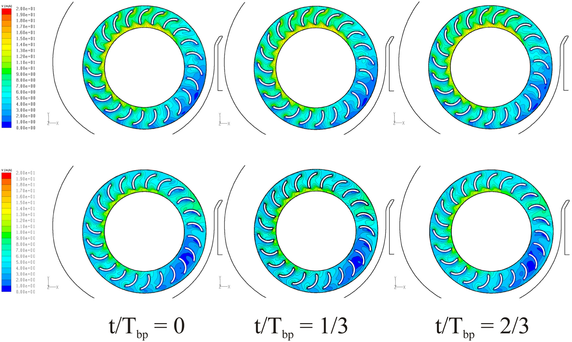
The averaged velocity fields give information of the steady performance of the fan blades, as a function of the relative to tongue position. However, for comparison of the two different operations, instantaneous velocity fields are considered and two different flow rates are considered. Figures 20 and 21 plot the unsteady velocity fields at three different times equally spaced on the blade passing period. The two flow rates are chosen considering the performance curves in Figure 17.

Figure 20.

Instantaneous velocity patterns in the impeller, φ = 0.359 (low flow rate).

Figure 21.

Instantaneous velocity patterns in the impeller, $\phi$  = 0.495 (close to nominal flow rate).

The first flow rate, in Figure 20, is chosen at a low flow rate, where separation problems are more likely to appear. The upper figures are for the baseline configurations, while the lower ones are for the blocked inlet fan. The lower velocity is found at a position around 30° from the volute tongue. Globally speaking, for the upper figures, a higher velocity is found in any position and a more uniform flow is found. For the lower figures (blocked inlet), a deeper low-velocity region is found at 30° after the volute tongue. Even a recirculation flow zone is found for t/T_bp = 1/3 and 2/3. However, it does not seem that the region where this is happening increases or differentiates one case from the other. Therefore, a more important separation zone is found giving rise to higher losses for the blocked inlet configuration. It must also be kept in mind that the flow rate condition is almost the same, but not the obtained pressure increase (Figure 17).

Figure 21 plots the second flow rate, around φ = 0.46 for the blocked inlet simulation and φ = 0.51 for the baseline one. Obviously, the region with lower velocity diminishes in comparison with previous figure. Again, in the comparison between the baseline and the blocked inlet operation, a smaller velocity decrease is found for the baseline one. At this flow rate, an increase in the low-velocity region is retrieved for the blocked inlet operation, meaning that the comparison between the two operations provides less meaning than in the previous figure, because the difference in pressure rise between the two operations is much higher for this flow rate, than for the lower one.

To complement the instantaneous velocity fields within the impeller, an equivalent study is developed for the volute. For such a purpose, a plane just downstream of the impeller and before the volute tongue is chosen. In that plane, two regions with different flow behaviour can be observed: one is the near-impeller exit region and the other is the volute region. In the following figures, those regions are clearly divided by a dash line, so that below that line, the near-impeller region will show more fluctuations and the volute region will show more uniform conditions, with less time fluctuations.

Figure 22 shows the time evolution of the velocity fluctuations for the mentioned plane in the volute and three different times that correspond to different blade-to-blade positions. On the right-hand side of the figure, the averaged or mean field has also been plotted. Two different scales are chosen, one for the velocity fluctuations and another one for the mean velocity. This representation is based on the following calculations

$$\{\begin{array}{c}\mathrm{Averaged\; velocity}:\overline{\mathrm{V}}=\frac{\overrightarrow{\mathrm{V}}}{\omega (D/2)}\\ \mathrm{Instantaneous\; velocity\; fluctuations}:100\frac{\overrightarrow{\mathrm{V}}-\overline{\mathrm{V}}}{\overline{\overline{\mathrm{V}}}},\mathrm{with}\overline{\overline{\mathrm{V}}}=\frac{\mathrm{Q}}{\mathrm{Lb}}.\end{array}$$

(4)

Figure 22.

Mean velocity and velocity fluctuations at different flow rates.

The velocity fluctuations, at any time, are within the range ±3%, while the averaged velocity is in the range [0, 1.1], for the three considered flow rates.

Increasing mean velocity values are found for increasing flow rates (Figure 22, right-hand side column). At the lower flow rate (φ = 0.359), a wide low-speed region is found in the averaged flow field with two even lower regions near the side walls. At the middle flow rate (φ = 0.495), close to the nominal one, the two side lower speed regions remain, but the region itself is smaller. The trend is also kept for the higher flow rate (φ = 0.766).

The fluctuating velocity field shows a common trend for the studied plane (left part of Figure 22), with higher variations in the region close to the impeller, below the dashed line. The rotating impeller blades are quite clearly shown for the different plotted time frames, namely, t/T_BP = 0.2, 0.5 and 0.8. Alternating positive and negative fluctuations are found for the two sides of the impeller blade passages that are in a staggered configuration. There are not many instantaneous differences for the different relative impeller positions and only residual changes are found. In the flow rate evolution, a minimum in the velocity fluctuations is found for a nominal flow rate, with increasing values for off-design conditions. The maximum velocity fluctuations are found at a higher flow rate.

With the numerical flow simulation results, a definition and mapping of the helicity is possible, following its definition as

$$\mathrm{Helicity}\equiv \mathcal{H}=(\nabla \times \overrightarrow{\mathrm{V}})·\overrightarrow{\mathrm{V}}$$

(5)

This variable provides information on the vorticity aligned with the stream flow and has been plotted here to identify secondary flows. Inside the impeller, and due to the momentum exchange, there is an increase in vorticity, but in the volute there should be a kind of vorticity conservation along the stream paths and subsequent vanishing effect.

Figure 23 shows the time evolution of the helicity fluctuations for the same plane in the volute and same conditions as the ones explained for Figure 22. On the right-hand side of the figure, the averaged or mean helicity field has also been plotted. Two different scales are chosen, one for the helicity fluctuations and another one for the mean or averaged helicity. The representation in Figure 23 is based on the following calculations

$$\{\begin{array}{c}\mathrm{Averaged\; helicity}:\overline{\mathcal{H}}=\frac{\overrightarrow{\mathcal{H}}}{\omega \overline{\overline{\mathrm{V}}}}\hfill \\ \multicolumn{1}{c}{\mathrm{Instantaneous\; helicity\; fluctuations}:100\frac{\overrightarrow{\mathcal{H}}-\overline{\mathcal{H}}}{\omega \overline{\overline{\mathrm{V}}}}}\end{array}$$

(6)

Figure 23.

Averaged helicity and fluctuations’ maps for the baseline operation and three different flow rates.

The helicity fluctuations, at any time, are within the range ±30%, while the averaged helicity is in the range [−7, 7], for the range of considered flow rates.

Apart from some secondary structures, a clear pair of contra-rotating vortices is found near the impeller exit region, for the whole range of studied flow rates. The relative strength of the vortices shows a decreasing trend with increasing flow rates.

About the instantaneous helicity fluctuations (left-hand side of Figure 23), it can be observed how those affect only the near-impeller region, with little or no effect on the second or volute region. Neither the strength of these fluctuations nor their values change much with different time steps, but there is a clear influence of the flow rate. Helicity fluctuations increase with increasing flow rate, and a clear maximum is found for a higher analysed value (φ = 0.766).

The time evolution of the helicity fluctuations shows a clear time dependence. For a lower flow rate (φ = 0.359, at the top of Figure 23), an almost constant pattern is found, with variations only in the middle plane, for each time instant. However, for increasing flow rates (φ = 0.495 and φ = 0.766, that is, the middle and bottom parts of Figure 23), the helicity fluctuations are placed on both sides of the middle plane. An explanation for this is that for increasing flow rates, the effect of the helicity due to the blade passing flow becomes predominant.

For the local losses or secondary flow effects, the important value is the helicity itself (right-hand side of Figure 23). Therefore, the attention has to be focused on the right-hand side averaged value. Then, the maximum losses due to secondary flows are located in the near-impeller region and are stronger for lower flow rates (in our study, for φ = 0.359).

Therefore, an increase in averaged helicity for decreasing flow rates is observed. In other words, the minimum of this averaged helicity is found for higher flow rate. In a global perspective, a pair of counter-rotating vortices with varying strength is found. This behaviour follows what was obtained in González and Santolaria ²⁷ for a centrifugal pump.

As a conclusion, and with varying strength as a function of the flow rate, a counter-rotating pair of vortices is found. Also, with a clear structure, a high mixing zone is found in the region near impeller.

Only the results for the baseline operation are shown, and any comparison here would be misleading to wrong conclusions as equivalent working points are not possibly achieved with the blocked inlet operation. Nevertheless, from the available data, it can be concluded that a higher level of averaged helicity is found, with almost similar patterns (quite similar to Figure 23), but as mentioned, no real comparison is possible.

Conclusion

The dynamic effects of the flow in a centrifugal fan have been studied both through a numerical flow study and by the experimental recording of vibration signals, following two perpendicular directions, the horizontal and vertical ones. Considering the experiments, a well-established fault diagnosis protocol, namely, the POD techniques, was considered to describe the fan operation and characterize it. In what refers to the numerical model, the results do complement the experiments widening the number of possible failures. The main goal of the study is then reached, namely, the survey to a series of possible and real operation failures of the fan unit.

The main conclusions of the experiments and POD analysis point that the highest vibration was found to be 2.5 times the gravitational acceleration, and it happens for the unbalance of the impeller fault. The lower one is always for the baseline operation at any flow rate, with a maximum of 0.3 times the gravitational acceleration. The obstructed channel configuration shows a quite different behaviour in comparison with the baseline and the unbalance of the impeller. A minimum of vibrations is found for the baseline operation and relatively high flow rates.

At off-design flow rates, the unbalance impeller fault results in higher accelerations, while for the nominal flow operation, both studied faults produce equivalent acceleration values.

Within a global frame, the study preludes a maintenance method for small centrifugal fans. The main fault diagnosis study performed gives already an idea of the main working range parameters and the possible fault detection procedures.

On the other hand, considering the numerical analysis and the blockage of the free inlet, for the global variables, an important shift in the performance curves when compared with the experimental data was found. However, the possibilities of the numerical model allow a detailed flow study, which was carried out.

For the inlet flow structure, a more equal flow division at both sides of the central plate is found when the flow rate increases. In parallel, an increase in flow separation for higher flow rates is observed. These conclusions are repeated for the two observed planes.

At the impeller, there is a quite marked difference between the free inlet and the obstructed one. The effect of the volute tongue is also clear at higher flow rates, with a less symmetric flow for lower and close to nominal operating conditions. In general, the low chord blades show relevant separated condition, especially at the outlet section (near the impeller outlet).

Finally, a section after the impeller outlet and just before the volute tongue is chosen to see the effect of the operation conditions on the discharged flow. At this section, the maximum velocity is obtained for the vicinity of the impeller. A typical vortex structure has also been obtained, increasing for higher flow rates, when the helicity fluctuation contours are considered. The plotting of the helicity in such a plane has revealed the relative effect of the middle plane in the flow structure.

After concluding the whole study, considering the four studied failures, the set of generated data provides a deep insight into a wide range of operation conditions for the fan. The observed results point to a relatively good aerodynamic performance for low and nominal conditions, while less uniform conditions are found for high flow rates. That is, less axi-symmetric flow in the impeller and a more important vortex flow structure in the discharge.