Simulation analysis of performances and yield rates on a lens module

Abstract

A simulation platform is developed to analyze the tolerance ability of designed lens in the opto-mechanical system. The major task of lens designer is to find out the optimal parameters to meet the specification requirement. A real lens with decenter, tilt, and lens parameters’ variation could lower the performance of lens. The original parameters from the lens designer suffer certain probability distribution during manufacturing lenses so that the performance of assembly lens is always different from that of the optimal design. The proposal applies a variety of probability density functions of the manufacture to obtain the tolerance parameters used in simulation. Some macros of commercial optical software based on the Monte Carlo method are developed to simulate the lens manufacture tolerance and analyze the yield rate for mass production. With proper probability density functions of the manufacture, the tolerance can be estimated from the proposed algorithm.

Introduction

Most initial lenses are designed under ideal condition without considering the lens variation during assembly. This would make the yield rate of lens hard to be promoted for mass lens production. The dimensional variations in the optics and mechanical elements are relative to fabricated accuracy, which stack-up the tolerance in real world. It is more reasonable for lens designer to predict the yield rate of a lens system before mass production. As a result, an interface^1–3 is necessary to manage the problem between the optics and mechanics during the optical system development.

An opto-mechanics is responsible for balancing the optics and mechanics to obtain acceptable tolerances in an optical system. The mechanical structure of the optical system is required to meet the lens specification, and also the necessary tolerance is required for satisfying the image quality. Such variations in radius, deflection, and displacement would degrade the distribution of yield rate in the lens assembly, and hence tolerance is a critical issue in lens design.^4,5 An opto-mechanical tolerance model was proposed ⁶ to calculate the element tilt, decenter, and despace stack-up within a cell. Some researches applied finite element analysis (FEA) ⁷ to simulate the assembly process for lens manufacture. Zia and Qiao ⁷ investigated the role of certain clearances in an assembly structure. Moreover, Monte Carlo analysis ⁸ is also widely applied to evaluate the optimum settings of the dimensions.

Predicting the yield rate is one of the most important objects for optics lens manufacture. The current optical software supports the simulation of optical quality that can vary the shape, location, tilt, and so on. The simulation results assign the accuracy of opto-mechanical structure. However, the crucial quality should be evaluated based on the assembly process and mechanical accuracy. The variations in mechanical increment would lead lens with tilt, decenter, and displacement to make the worst performance. Most optical software runs the tolerance analysis without considering the probability density function (PDF) in real situation, which results in the conflict between the lens design and manufacture. In this article, the common PDFs in real lens manufacture are applied to simulate a variety of tolerances used in the evaluation of yield rate. The PDF from the real statistical results of manufacture can improve the precision of tolerance analysis.

Some macros based on the Monte Carlo method are developed in the proposal to simulate the tolerance for evaluation of the yield rate during mass production. The tolerances from proper PDFs link to the parameters of original lens to obtain tolerance analysis with root mean square (RMS) spot size and modulation transfer function (MTF). As a result, the proposal provides an effective method to analyze the tolerance for lens mass production. The article is organized as follows. Section “Tolerance distribution in lens manufacture” describes the tolerance distribution in lens manufacture. Section “Random variable transformation from uniform distribution” illustrates how to transform the random variable from uniform distribution to desirable PDF. The simulation results are discussed in section “Simulation result and discussion.” Section “Conclusion” concludes this article.

Tolerance distribution in lens manufacture

A tolerance analysis^9,10 is an important process to estimate the product quality and cost for industrial development. Using tolerance analysis based on the manufacture limit could not only improve the quality of product but also lower the cost in mass production. An ideal lens system is to promise the assembly without any deviations as shown in Figure 1(a). However, real lens assembly suffers some variations like tilt and decenter on each component, as shown in Figure 1(b). There are many variations (e.g. vibration, material, temperature, residual stress of component) influencing the accuracy in a lens system, so we should determine the acceptable tolerances for components. Observing the accuracy from manufacture finds that the tolerance has some probability distributions, which could be classified into some well-known PDFs, f(x).

Figure 1.

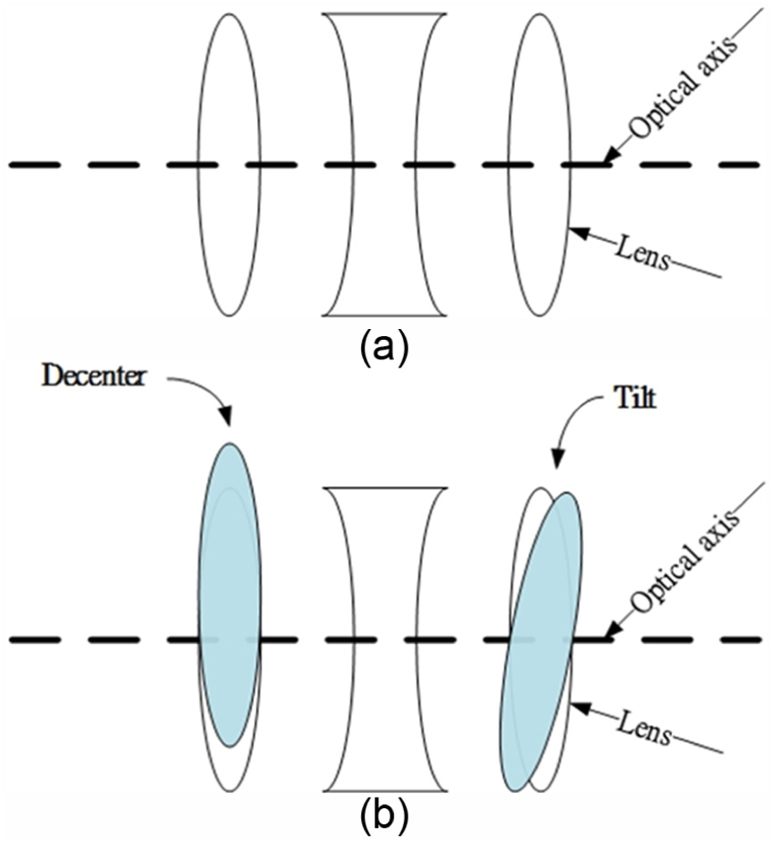
Optical lens assembly in (a) ideal situation and (b) real situation.

The behavior of general assembly process is like normal distribution for the deviations with tilt, decenter, and position. The lens shown in Figure 2 experiences the deviations with the tilt and the decenter being z_t and z_d, respectively. These two deviations can be expected according to probability statistics. Let Z be the random variable from some PDFs. For assembly process, we usually predict that there are no variations for tilt and decenter in lens system, indicating the probability of tolerance would be maximum at Z = 0 as shown in Figure 2. The probability is decreased as a lens system suffers more deviation so that the common tolerance of assembly process could be presented by normal distribution, as shown in Figure 3. The PDF of normal distribution is represented as follows

$$f(x)=\frac{e^{-{(x-m)}^2/2{\sigma }^2}}{\sqrt{2\pi }\sigma }-\infty <x<\infty$$

(1)

where m is the mean that is the original parameter of lens without suffering any tolerances, and σ is the variance that can be expressed as a range of tolerance.

Figure 2.

Relationship between random variable Z in lens system.

Figure 3.

The PDF of normal distribution.

Although current technologies could produce high accurate components for a lens system, it is difficult to maintain the same type of components without any tolerance during mass manufacture. Inspecting the variation in the radius discovers that the outcome is like Rayleigh distribution for lens element, ⁹ as shown in Figure 4. The convex radius grows large while the concave radius tends to be small during mass production of the lens elements. Therefore, Rayleigh distribution is applied to imitate the variations in the radiuses in both cases. Figure 5 shows the PDF of Rayleigh distribution. Its PDF is defined as

$$f(x)=\frac{x}{{\alpha }^2}{e}^{-x^2/2{\alpha }^2},x\ge 0,\alpha >0$$

(2)

Figure 4.

The distribution of the variations for lens radiuses.

Figure 5.

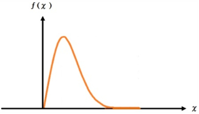
The PDF of Rayleigh distribution.

The mean of Rayleigh distribution is $\alpha \sqrt{\pi /2}$ .

The tolerance in lens manufacture has some features that can be statistical in an appropriate probability distribution. As a result, the random variable from proper PDF is applied to generate the variations in the tilt, decenter, thickness, curvature, and so on. However, common software only provides the random variable with uniform distribution, as shown in Figure 6. The random variables from a to b have the same probability 1/(b − a), which is defined as

$$f(x)=\{\begin{array}{c}\frac{1}{b-a}\mathrm{for}a\le x\le b\hfill \\ \multicolumn{1}{c}{0\mathrm{elsewhere}}\end{array}$$

(3)

Therefore, a transformation must be done from the uniform random variable to correspond the random variable of the PDF. The behavior of general assembly process is like normal distribution for the deviations with tilt, decenter, and position, while inspecting the variation in the radius discovers that the outcome is like Rayleigh distribution for lens element. Therefore, normal and Rayleigh distributions are applied to implement tolerance analysis in this article. However, the users can apply other PDFs from the real statistical results to implement tolerance analysis.

Figure 6.

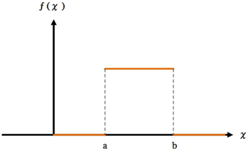
The PDF of uniform distribution.

Random variable transformation from uniform distribution

The random variables from proper PDFs are regarded as the variations in providing tolerance analysis. It is often difficult to generate these random variables directly, while a random variable from 0 to 1 with uniform distribution is always supported by common software. Therefore, we need to convert the possible variations in lens from uniform distribution for analyzing the lens. As we know, the relationship between the PDF and the cumulative distribution function (CDF; F(x)) can be expressed as

$$F(Z)=\underset{-\infty }{\overset{Z}{\int }}f(x)\mathrm{dx}$$

(4)

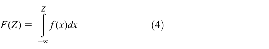
The range of all the CDFs is from 0 to 1, which is the same as the random variable in uniform distribution. The random variables transformed between two different PDFs can be executed by setting the two CDFs F_X(x) and F_Y(y) with same probability, that is

$$F_X(x)=F_Y(y)$$

(5)

where y is the function of x. From equation (5), we know that the relationship between uniform and normal distributions can be expressed as

$$U=F(Z)=\underset{-\infty }{\overset{Z}{\int }}\frac{1}{\sqrt{2\pi }\sigma }{e}^{-{(x-m)}^2/2{\sigma }^2}\mathrm{dx}$$

(6)

where U is the random value from 0 to 1 generated by the computer, and Z is the random variable of normal distribution. Figure 7 illustrates the relationship between uniform and normal distributions. When the random variable with uniform distribution is generated in the computer, the corresponding CDF is also determined, for example, the blue area shown in Figure 7. Because the transformation in equation (6) requires the same CDF, the red area must be the same as the blue area shown in Figure 7. The red area is cut off by the random variable Z with normal distribution so that the random variable Z can be found from equation (6).

Figure 7.

The relationship between uniform and normal distributions.

We understand that the random variable Z in equation (6) can be found from F⁻¹(U). However, we cannot deduce equation (6) to find the random variable Z directly due to including the form of error function erf(x) for the derivation. The error function erf(x) is defined as

$$\mathrm{erf}(x)=\frac{2}{\sqrt{\pi }}\underset{0}{\overset{x}{\int }}{e}^{-t^2}\mathrm{dt}$$

(7)

Let

$$t=\frac{(x-m)}{\sqrt{2}\sigma },\mathrm{dt}=\frac{\mathrm{dx}}{\sqrt{2}\sigma }$$

(8)

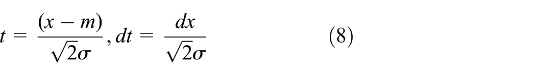
Equation (6) becomes

$$\begin{array}{cc}\multicolumn{1}{c}{U}& =\underset{-\infty }{\overset{(Z-m)/\sqrt{2}\sigma }{\int }}\frac{1}{\sqrt{\pi }}{e}^{-t^2}\mathrm{dt}\hfill \\ \multicolumn{1}{c}{}& =\frac{1}{2}\underset{0}{\overset{(Z-m)/\sqrt{2}\sigma }{\int }}\frac{2}{\sqrt{\pi }}{e}^{-t^2}\mathrm{dt}-\frac{1}{2}\underset{0}{\overset{-\infty }{\int }}\frac{2}{\sqrt{\pi }}{e}^{-t^2}\mathrm{dt}\hfill \\ \multicolumn{1}{c}{}& =\frac{1}{2}\mathrm{erf}\left(\frac{(Z-m)}{\sqrt{2}\sigma }\right)+\frac{1}{2}\hfill \end{array}$$

(9)

Finally, we can obtain the inverse equation

$$Z=\sqrt{2}\sigma \mathrm{er}{\mathrm{f}}^{-1}[2(U-0.5)]+m$$

(10)

The inverse error function efr⁻¹(x) could be approached as ¹¹

$$\begin{array}{l}{\mathrm{erf}}^{-1}(x)\approx \mathrm{sgn}(x)\\ \sqrt{\sqrt{{\left(\frac{2}{\pi a}+\frac{\ln (1-x^2)}{2}\right)}^2-\frac{\ln (1-x^2)}{a}}-\left(\frac{2}{\pi a}+\frac{\ln (1-x^2)}{2}\right)}\end{array}$$

(11)

where a = 0.147. Another possible distribution, Rayleigh distribution, can also be obtained from uniform distribution, that is

$$\begin{array}{c}\multicolumn{1}{c}{U=\underset{0}{\overset{Z}{\int }}\frac{x}{{\alpha }^2}{e}^{-x^2/2{\alpha }^2}\mathrm{dx}}\\ \multicolumn{1}{c}{=1-e^{-Z^2/2{\alpha }^2}}\end{array}$$

(12)

Then, the random variable of Rayleigh distribution is

$$Z=\sqrt{-2{\alpha }^2\ln (1-U)}$$

(13)

We can generate the corresponding random variables by equations (10) and (13) for tolerance simulation in real lens manufacturers.

Simulation result and discussion

The work of most lens designs is to find out the optimal refractive index, curvature, thickness, and aspherical coefficient. When the material of the lens is determined in the lens design, tolerance analysis is related to curvature, thickness, aspherical coefficient, tilt, and decenter. Except the refractive index, the other factors are considered to implement tolerance analysis in this article. Therefore, a complex lens can also implement tolerance analysis by the proposed method. A random variable transformation function is developed in the macros of optical software Code V in the proposal. There are 1 million random variables of uniform distribution generated to verify the PDFs of normal and Rayleigh distributions. Figure 8 shows the simulation results for the random variable transformation of normal and Rayleigh distributions from uniform distribution. As we can see, the distributions shown in Figure 8 are much similar to normal and Rayleigh distributions, respectively. Therefore, we can apply equations (10) and (13) to simulate tolerance analysis during mass production.

Figure 8.

The simulation of PDF in Code V for (a) normal distribution and (b) Rayleigh distribution.

The transforming random variables are regarded as the lens parameters in tilt, decenter, radius, and thickness. A mobile phone camera with 1 megapixel is used to implement tolerance analysis in the proposal. Figure 9 shows the layout of mobile phone camera. The fields of view (FOVs) are set as 0°, 11°, and 21°, and the f-number is set to 2.8. Table 1 lists the parameters of the lens, and Table 2 shows its aspherical coefficients. The first lens element is made of glass material while the other two are made of plastic. Four aspherical surfaces are used on the plastic materials to upgrade the lens performance. Figure 10 shows the spot diagram. The maximum RMS spot is around 6.7 µm at the FOV of 21°, resulting in the MTF larger than 0.4 at 100 lps/mm, as shown in Figure 11.

Figure 9.

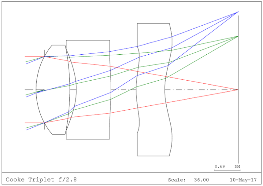
The layout of mobile phone lens.

Table 1.

Original parameters of the simulation lens.

Surface	Surface type	Y radius	Thickness	Glass
Object	Sphere	$\infty$	$\infty$
Stop	Sphere	$\infty$	−0.2252
2	Sphere	1.8769	0.9191	BSL7_OHA
3	Sphere	−5.7121	0.1762
4	Asphere	−1.8175	0.9409	PMMA_SPE
5	Asphere	−8.2936	0.6859
6	Asphere	2.3522	0.7779	PMMA_SPE
7	Asphere	1.9827	2.0000
Image	Sphere	$\infty$	0.0000

Table 2.

The aspherical coefficients of mobile phone camera.

Surface	4	5	6	7
A4	0.0632	0.0018	−0.1390	−0.1031
A6	0.0015	0.0243	0.0054	0.0017
A8	0.0000	0.0000	−0.0102	0.0000

Figure 10.

The spot diagram.

Figure 11.

The modulation transfer function (MTF).

All thicknesses in Table 1 and aspherical coefficients are used as the mean of normal distribution to find the appropriate variations while Rayleigh distribution is applied in the radiuses of the lens. Moreover, the zero mean is expected to tilt and decenter with normal distribution. Table 3 shows the corresponding PDFs used and common manufacture limit ¹ for the lens parameters. A program based on Tables 1 and 2 is developed to simulate for tolerance analysis. There are 10,000 individual lenses created with parameter variations for estimating the CDFs of RMS spot size and MTF.

Table 3.

The tolerances and distributions of the simulation.

	Tolerance	Distribution
Tilt	1 arcmin	Gaussian
Decenter	50 µm	Gaussian
Thickness	50 µm	Gaussian
Radius of curvature	0.10%	Rayleigh
Coefficient of aspheric lens	0.01	Gaussian

According to tolerance distribution in Table 3, Figure 12 shows the CDF of the RMS spot size and MTF at 100 lps/mm. The 100% yield rate requires a spot size larger than 200 µm, which is much larger than the optimal one (about 6.7 µm). Figure 12(b) shows the yield rate to be around 1% for MTF 0.2 under 100 lps/mm. The results could not be acceptable for manufacturing. Since the modern mobile phone lenses use numerous aspherical surfaces to upgrade the image quality, they need to suffer more tolerance constraints during the manufacture. Today, the fabricated precision of the mobile phone lens has been promoted 10 times of traditional tolerance distribution (Table 3).

Figure 12.

The simulation result based on normal tolerance constraint: (a) RMS spot size (mm) and (b) MTF value at 100 lps/mm.

Figure 13 shows the CDF of the RMS spot size and MTF at 100 lps/mm by promoting the precision 10 times of Table 3. As we can see, the spot size can be improved to less than 25 µm when requiring 100% yield rate, as shown in Figure 13(a). Under 100 lps/mm, there are around 60% of lens that can be satisfied as the MTF required is larger than 0.2. It is more acceptable for the lens manufacture. As a result, the tolerance analysis shows that the results are close to the real lens manufacture for mobile phone. Using the proposed algorithm can effectively predict the yield rate for mass manufacture.

Figure 13.

The simulation result based on small tolerance constraint: (a) RMS spot size (mm) and (b) MTF value at 100 lps/mm.

Conclusion

A preliminary platform of tolerance analysis has been proposed in this article. The real PDFs of mechanical assembly (e.g. normal and Rayleigh distributions) are considered in tolerance simulation. The PDFs are generated from uniform distribution by developing the macros in Code V so that the generated random variables could be regarded as tilt, decenter, and thickness of lens in tolerance analysis. There are 10,000 individual lenses with tolerance from the generated random variables for estimating the CDF of the RMS spot size and the MTF. The simulation results show that the yield rate could not be acceptable for common tolerance distribution. However, the precision of lens fabrication could be less than 5 µm for the assembly process, which improves the yield rate during mass production. The results show that there are around 60% of fabricated lenses satisfying for MTF 0.2 under 100 lps/mm. As a result, the tolerance analysis is close to the yield rate of lens manufacture for mobile phones. Therefore, using the proposed scheme can remarkably predict the yield rate of lens during mass production.