A research into the flow and vortex structures around vehicles during overtaking maneuver with lift force included

Abstract

A simulation model of overtaking maneuvers is established to research into the flow and vortex structures around two identical Ahmed vehicles. The simulation demonstrates how the flow and vortex structures generate and change, which influences the aerodynamical coefficients of the vehicles most. In this study, a transient solver is used on the platform of ANSYS/Fluent, and the sliding mesh method is adopted to simulate the motion of the overtaking vehicle, which realizes a more actual recovery of the road conditions. Based on the fact that the primary factor that influences the aerodynamical coefficients of a vehicle is the change in the outer flow around it, a research into the variation in the outer flow field is conducive to in-depth analysis of the aerodynamical characteristics of the vehicle. Most previous studies focused only on the lateral aerodynamical coefficients during overtaking maneuvers. This article establishes a comprehensive model that takes the lift force into consideration to more accurately simulate the aerodynamical characteristics. Moreover, it is aimed at figuring out the key factors that cause the change in the aerodynamical coefficients at vortex level in this study, not just at pressure level as most previous studies did.

Introduction

It has been proven by previous studies that the magnitude of lift force is positively correlated to the vehicle speed. ¹ This explains why the adhesion force of a vehicle reduces when it is traveling at high speed. And this is one of the potential risks of high-speed driving.

Moreover, when a vehicle overtakes another at high speed, the flow fields of the vehicles change dramatically, resulting in the fluctuation of the vehicle aerodynamic coefficients. Consequently, the two vehicles tend to get close to each other and lift up away from the road surface. What is more severe is that the interaction of the flow field around the two vehicles reduces the threshold velocity under which the vehicles lift up away from the road, that is, the adhesion force reducing to zero. These influences will slow down the response of the steering system and cause the drivers to misestimate the road conditions or even misoperate, which sharply increases the driving dangers.

There have been a lot of studies on aerodynamical coefficients of vehicles during the overtaking maneuvers in the past decades. Noger et al. ² analyzed most of the factors which influence the aerodynamical coefficients through wind tunnel tests, such as the relative velocity, lateral space, and yaw angles. The test results were comprehensive and valuable and provided a reliable standard for subsequent studies including this article. On the basis of Noger et al.’s ² study, Uystepruyst and Krajnović ³ conducted overtaking simulations with sliding mesh method using commercial fluent software. They particularly explained the variations in lateral aerodynamical coefficients during overtaking maneuver stage by stage and figured out what caused these variations using pressure field figures and streamline figures. Corin et al. ⁴ compared the accuracy difference between quasi-steady method and sliding mesh method and finally verified the reliability of the results of sliding mesh method during overtaking maneuvers. This article takes a step further and undertakes independent researches into the front high-pressure region and rear low-pressure region of the vehicles to obtain more detailed results than Corin et al.’s ⁴ article.

Besides the researches on the overtaking maneuvers of two identical vehicles, there are other researches about two different vehicles. Yamamoto et al. ⁵ and Howell and colleagues^6–8 researched into the overtaking maneuvers of a bus and a car. The model in Yamamoto et al.’s ⁵ article was established to research into a bus overtaking a car in transient wind tunnel tests, and then the aerodynamical influence of the bus on the stability of the car was discussed. The model in Howell et al.’s ⁷ article was established to research into a car overtaking a bus in quasi-steady wind tunnel tests. Similarly, the influences of lateral space and yaw angle of the car were discussed with the six-component results of the car.

As a general trend in vehicle design, lightweight significantly helps reduce fuel consumption and cost. However, it makes the influence of lift force on stability and safety of vehicles at the same time. This article researches into the influences of lift force during the overtaking maneuvers which have been paid little attention to in previous researches while important to lightweight vehicles and moves a forward step to analyze the reasons of the variation in the six-component and the surface pressure on vertex level. This study is an extension of Uystepruyst and Krajnović’s ³ research.

Description of the geometry and the wake flows

The geometry used in this study is identical to that in Uystepruyst and Krajnović, ³ and it is a 7/10 Ahmed body with a slant angle of 30°, as shown in Figure 1. This body was chosen because of its relatively simple topology which simplifies the generation of the grid for numerical predictions while maintaining all typical characteristics of the flow field around a passenger car. ¹⁰ Therefore, the simulation based on Ahmed model conducted in this article can represent a general category of overtaking maneuvers of two passenger cars.

Figure 1.

7/10 Scale Ahmed bluff body^3,9 (dimensions in mm).

Both bodies are characterized by a round front and a sharp rear. The main vehicle dimensions are shown in Figure 1. The Reynolds number based on the length of the vehicle is $\mathrm{Re}=1.5\times 10^6$ , at the velocity of 30 m/s. The wake flows of the Ahmed vehicle adopted in this article are three-layer vortex system, as shown in Figure 2.

Figure 2.

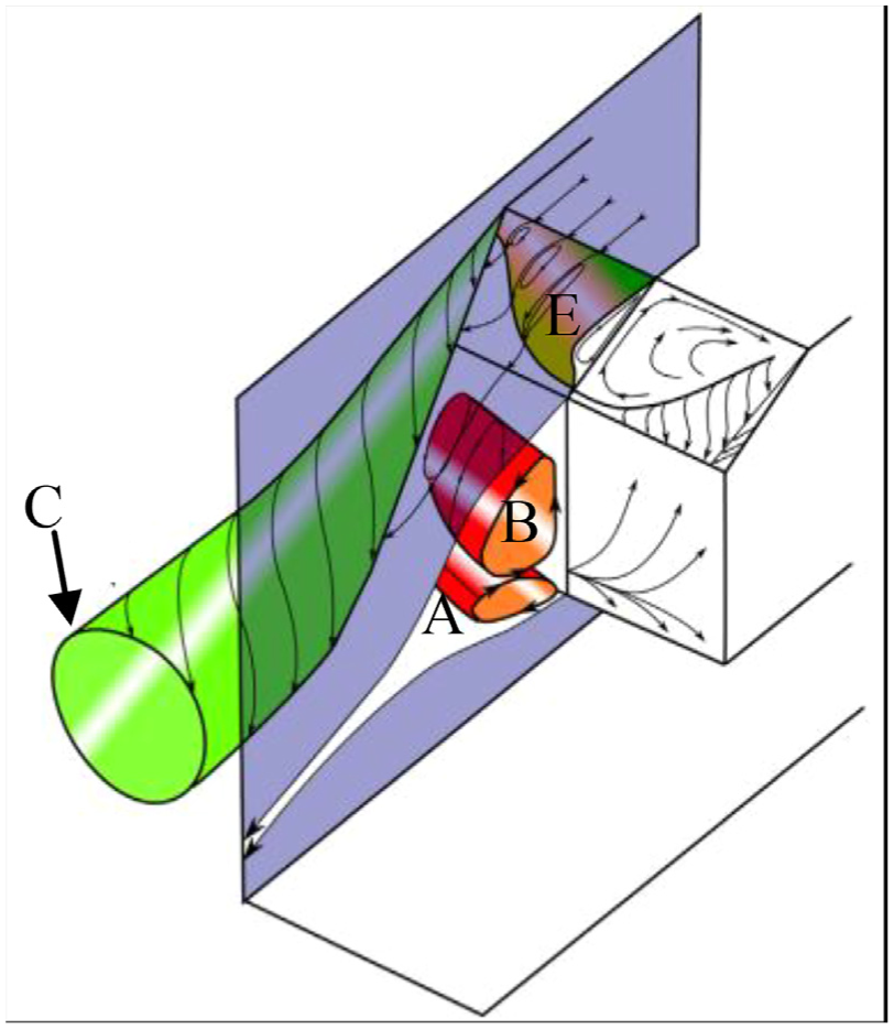
Vortex system of models in this article. ¹¹

The outer layer is the trailing vortex C. The middle layer can be divided into two toroidal vortices. Vortex A from the bottom of the vehicle is anti-clockwise while Vortex B from the roof of the vehicle is clockwise. And the high circumferential velocities of A and B indicate high velocity and low pressure of the flows underneath and above the vehicle.

The inner layer, separation bubble E, is observed in a flow regime while the flow is close to reverting back to the square back flow pattern. Then the separated flow reattaches on the slant. As a result, when the vortex structure is formed on the slant, the pressure on it declines. ¹²

Coordinate system and non-dimensional coefficients

For meaningful comparison between datasets, the pressure, force, and moment coefficients were nondimensionalized according to the following formulas

$$\{\begin{array}{c}{C}_d=\frac{2D}{\rho S{V}^2}\hfill \\ \multicolumn{1}{c}{C_s=\frac{2Y}{\rho S{V}^2}}\\ \multicolumn{1}{c}{C_l=\frac{2L}{\rho S{V}^2}}\\ \multicolumn{1}{c}{C_m=\frac{2N}{\rho \mathrm{lS}{V}^2}}\\ \multicolumn{1}{c}{C_{\mathrm{pm}}=\frac{2P}{\rho \mathrm{lS}{V}^2}}\\ \multicolumn{1}{c}{C_p=\frac{2(p(s)-p_{\infty })}{\rho V^2}}\end{array}$$

(1)

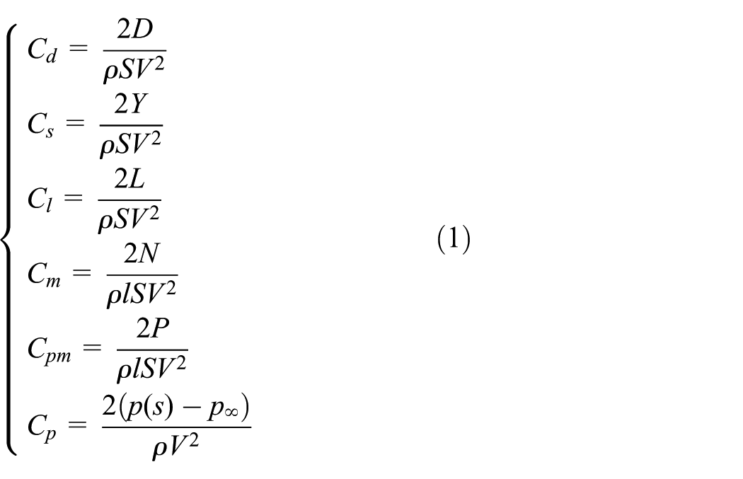
where C_p, C_d, C_y, C_l, C_m, and C_pm are the pressure coefficient, drag force coefficient, side force coefficient, lift force coefficient, yaw moment coefficient, and pitching moment coefficient, respectively. Correspondingly, D, Y, L, N, and P are the drag force, side force, lift force, yaw moment, and the pitching moment obtained by integrating the pressure distribution and shear stress distribution over the model surface, ¹ respectively. ρ is the air density, S is the body frontal area, and l is the longitudinal distance between the supports (wheel base). V is the steady velocity

$$V=V_{\infty }+V_r$$

(2)

where $V_{\infty }$ and $V_r$ are defined in Figure 2. $V_{\infty }$ is the freestream velocity. V_r is the relative velocity; in other words, the velocity difference between the two vehicles.

Computational simulation approach

Computational grid design

Unstructured grids are generated using the commercial grid generator ANSYS ICEM and consist of only tetrahedral elements. Three kinds of grid densities are designed in this article, and the parameters of them are shown in Table 1. Y⁺ is the distance between the mass center of the first layer grids and the wall, which is correlated to the velocity, viscosity, shear stress, and so on. The ranges of Y⁺ recommended by different researchers are different. According to Aljure et al.’s ¹³ research, Y⁺ is set to 40, 30, and 20, respectively, and the initial height of the boundary layer grids is estimated by the calculator. ¹⁴ Then, the height ratio is set to 1.2, and the number of layers is set to 10. The total elements are also shown in Table 1.

Table 1.

The parameters of the grids.

	Y+	Initial height of boundary layer grids (mm)	Total elements
Coarse	40	0.4713	92,000
Middle	30	0.3534	143,000
Fine	20	0.2356	201,000

Numerical methodology

This is a pressure-based dynamic simulation, which uses the realizable k–ε turbulence model^15–17 and a non-equilibrium wall function. And the second-order implicit temporal scheme based on the semi-implicit method for pressure-linked equations (SIMPLE) method is established in this article. A second-order upwind scheme was used to discretize the momentum, the turbulent kinetic energy, and the turbulent dissipation rate. ¹²

The computational domain of the overtaking simulation is shown in Figure 3.The overall domain is composed of two subdomains:

• Body1, containing the stationary vehicle Car1 which remains fixed during simulation

• Body2, containing the moving vehicle Car2 which moves with Car2 at the same velocity

Figure 3.

Notations for the location and the dimensions of the computational domains during the overtaking maneuvers (units in m).

The dimensions of the two subdomains are set as in Uystepruyst and Krajnović. ³ The length is 8 m, the width is 1.5 m, and the height is 1.5 m. The distance between the nose of the car and the inlet is 3 m. The positions of the inlets and outlets are shown in Figure 3. The boundary conditions are shown in Table 2.

Table 2.

Boundary conditions.

	Car1	Car2
Inlet	Velocity, $V_{\infty }=30\mathrm{m}/\mathrm{s}$	Velocity, $V_{\infty }=30\mathrm{m}/\mathrm{s}$
Outlet	Pressure, P = 0	Pressure, P = 0
Floor	Moving wall, $V_{\infty }=30\mathrm{m}/\mathrm{s}$	Moving wall, $V_{\infty }=30\mathrm{m}/\mathrm{s}$
Roof	Symmetry	Symmetry
Car body	Stationary wall	Moving wall, Vr
Adjacent surface	Interface	Interface
Outer side surface	Symmetry	Symmetry

The procedure of numerical computation

There are many simulation conditions in this article, but the computational analysis procedures under different conditions are basically the same.

Taking V_r = 10 m/s, Y/W = 0.25 as an example, Car2 and Body2 are placed behind Car1, and the distance between the front of vehicles is 2.5L (L is the length of the vehicle). Then, a steady-state simulation is conducted at this position, and the convergence results are taken as the initial state of the transient simulation. Time step size of the transient simulation is set to 1 × e⁻⁵ s. After 7320 time steps, Car2 reaches Location 1.5 after which the interaction of the flow fields can be ignored, representing the end of the overtaking maneuver. To simulate the entire flow fields during the overtaking maneuver, an interface between Body1 and Body2 is established to exchange data in the flow fields. The calculations are finished after 31,600 time steps when Car2 is 2L before Car1. To obtain more reliable results, the comparative data are taken only from Location −1.5 to Location 1.5, as shown in Figure 3.

Numerical results of the aerodynamic parameters during the overtaking maneuvers

Simulation validity verification

Numerical accuracy is checked by comparing the aerodynamical coefficients of the overtaken body in the simulation to the experimental data ² in the case of V_r = 10 m/s, Y/W = 0.25. C_y and C_m calculated from the three meshes are shown in Figure 4. The results of coarse grids involve overestimations of peak values of C_y and C_m, while the results of middle and fine grids are close to the experimental data, which means the middle and fine grids are convergent. Therefore, the middle grids are chosen for subsequent simulations. The surface, volume, and boundary layer grids of the vehicles are shown in Figure 5; the plot of Y⁺ which is obtained from the convergent simulation is shown in Figure 6; the maximum, minimum, and mean values are shown in Table 3.

Figure 4.

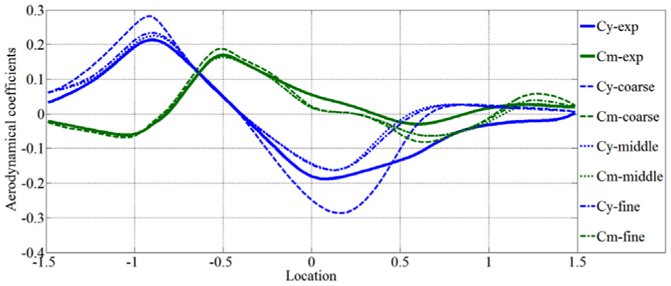
The comparison of aerodynamical coefficients.

Figure 5.

Surface and volume grids of bluff body.

Figure 6.

The plot of $Y^{+}$ of the two vehicles.

Table 3.

The maximum, minimum, and mean values of Y⁺.

	Maximum	Minimum	Mean value
Car1	33	0.76	16.5
Car2	44	1.05	24.5

C_y is relatively close to the experimental data in the first half as shown in Figure 4. At the first peak of C_y, occurring at Location −1, the difference between the experimental data and the numerical data is +10%, while at the first peak of C_m the difference is 5.5%.

The initial state of the flow fields

Figure 7 shows the pressure contour and the isosurface of the flow fields when the lateral distance between the two vehicles is far enough. The flow fields around the two vehicles are no longer influenced by each other, and the two flow fields are identical. The flow surrounding the stagnation region in front of the car is shown in the velocity isosurface. The velocity in Body1 is 25 m/s, and the velocity in Body2 is 35 m/s when V_r is 10 m/s. The trailing vortices are shown in Q-isosurface, Q = 200.^13,18 The background is the pressure contour on the plane of mass center, and the pressure ranges from −1055 to 547 Pa.

Figure 7.

The pressure contour and the isosurface of velocity and Q criterion to extract vortices.

To clarify the variation in the flow fields, the two sides of the vehicles are distinguished as the inner side and outer side, as shown in Figure 7. And the flows around the vehicles are named as listed in Table 4. Figures 8 and 9 show the vorticity and velocity of the initial flow fields, respectively.

Table 4.

The names of the flow around the vehicles.

Name	Flow	Name	Flow
L 1	Flow surrounding the stagnation region in front of Car1	L 2	Flow surrounding the stagnation region in front of Car2
O1	Flow on the outer side of Car1	O2	Flow on the outer side of Car2
I 1	Flow on the inner side of Car1	I 2	Flow on the inner side of Car2
C 1	Trailing vortices on the outer side of Car1	C 1	Trailing vortices on the outer side of Car2
D 1	Trailing vortices on the inner side of Car1	D 2	Trailing vortices on the inner side of Car2
E 1	Vortex on the slant of Car1	E 2	Vortex on the slant of Car2
A 1	Vortex A in Figure 2 of Car1	A 2	Vortex A in Figure 2 of Car2
B 1	Vortex B in Figure 2 of Car1	B 2	Vortex B in Figure 2 of Car2

Figure 8.

The vorticity of the initial flow fields.

Figure 9.

The velocity of the initial flow fields.

The aerodynamical coefficients of the vehicles are shown in Table 5. C_y and C_m should be zero in ideal condition, but they are not here due to the simulation error which is acceptable.

Table 5.

The initial aerodynamical coefficients.

Aerodynamical coefficients	Cd	Cy	Cl	Cm	Cpm
Numerical value	−0.31	0.002	0.36	−0.004	−0.103

The influence of lateral space on the aerodynamical coefficients during overtaking maneuver

Figure 10 demonstrates the influences of different lateral spaces on all aerodynamical coefficients when V_r = 10 m/s. It is shown in Figure 10 that the trends of the curves are roughly consistent while the amplitudes of the curves show differences.

Figure 10.

Aerodynamical coefficients during the overtaking maneuvers: (a) drag coefficients, (b) side force coefficients, (c) yaw moment coefficients, (d) lift coefficients, and (e) pitching moment coefficients.

Kim and Kim ¹⁹ researched into the variation in drag force coefficient in different lateral spaces. However, the lateral spaces influence not only the drag force coefficient but also the amplitudes and peak positions of many aerodynamical coefficients. The influences of the lateral space on the amplitude of the aerodynamical coefficients of the two vehicles are roughly the same. That is, the absolute values of aerodynamical coefficients are negatively correlated to the lateral space. Then as to the peak positions, the influences of the lateral space are different. For Car1, the lateral space has little influence on the peak positions of its aerodynamical coefficients. However, for Car2, the peak positions move backward as the lateral space decreases.

The influences of the relative velocity on the aerodynamical coefficients

Besides the lateral space, the relative velocity also has dramatic influences on the flow fields during the overtaking maneuvers. The curves of the aerodynamical coefficients in V_r = 5 m/s, V_r = 10 m/s, V_r = 15 m/s, and V_r = 20 m/s when Y/W = 0.25 are shown in Figure 11.

Figure 11.

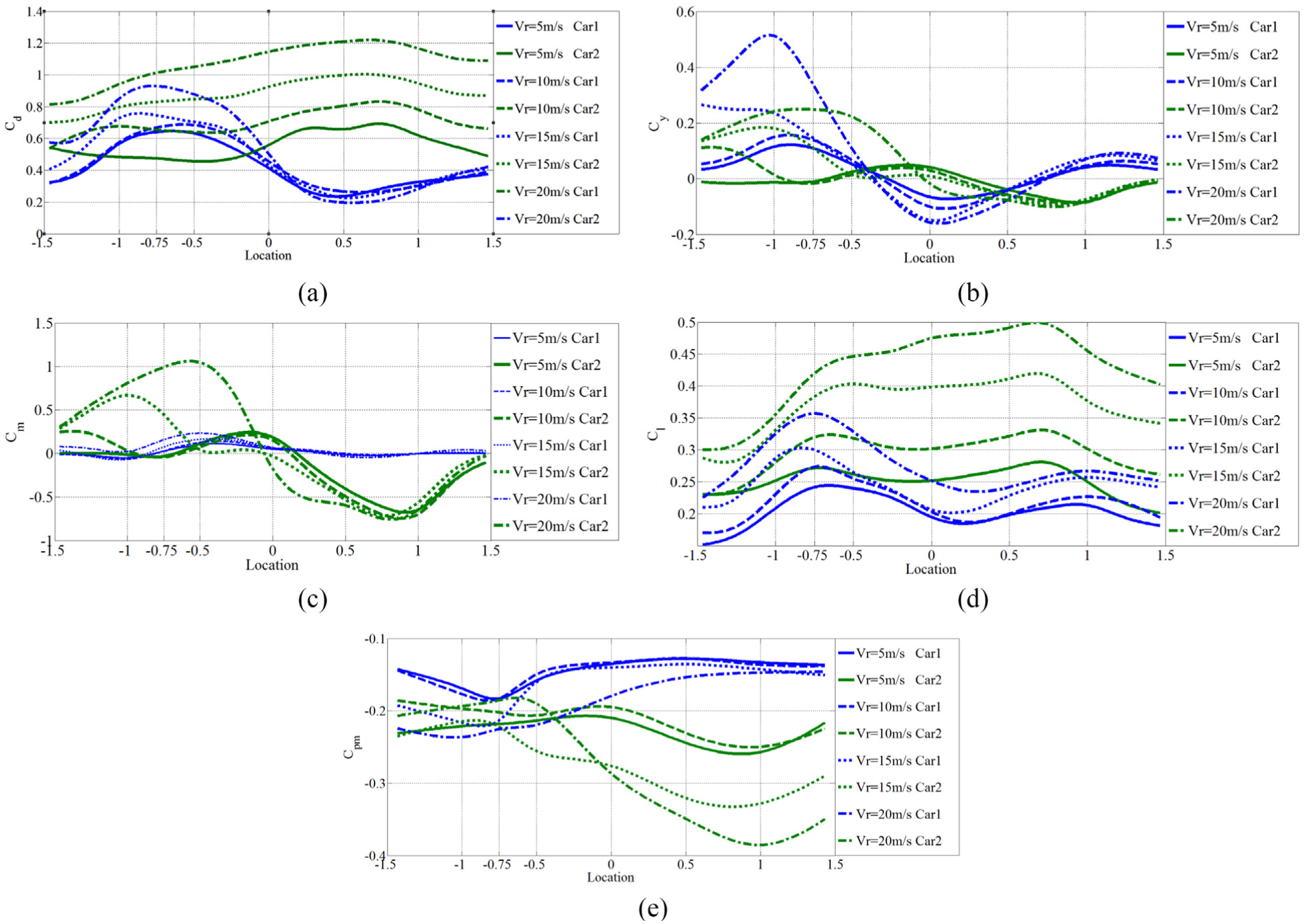
Aerodynamical coefficient curves at different relative velocities: (a) drag force curves at different relative velocities, (b) side force curves at different relative velocities, (c) yaw moment curves at different relative velocities, (d) lift force curves at different relative velocities, and (e) pitching moment at different relative velocities.

The variation tendencies of the longitudinal coefficients (C_d, C_l, and C_pm) of both vehicles are roughly the same. The peak positions of the curves for both vehicles remain fixed at different relative velocities while the absolute values of these coefficients are positively correlated to V_r.

The variations in the lateral coefficients—C_y and C_m—of both vehicles are different. The variations in lateral coefficients of Car1 are the same as that of the longitudinal coefficients. However, the variations in lateral coefficients of Car2 show different characteristics before and after Location 0. Before Location 0, V_r delays the appearance of the first peak, and the absolute values of C_y and C_m are positively correlated to V_r. After Location 0, the influence of V_r on the lateral coefficients decreases, and the curves of different V_r get close.

The velocity of the flow fields

It is observed from Figures 9 and 12(a) that the velocities of B₂, C₂, D₁, and D₂ increase when the overtaking maneuvers begin. With the movement of Car2, the velocity of D₁ continuously increases. Until Car2 moves to Location −0.75, D₁ and D₂ start to interact and combine with each other. They move together as a combining vortex pair. The combining vortex pair is named as C′, which contains a pair of counter rotating vortices, as shown in Figure 13. With the movement of Car2, the velocity of C′ increases and reaches its maximum at Location 0. After this location, the two vehicles start to separate, and the velocity of C′ decreases.

Figure 12.

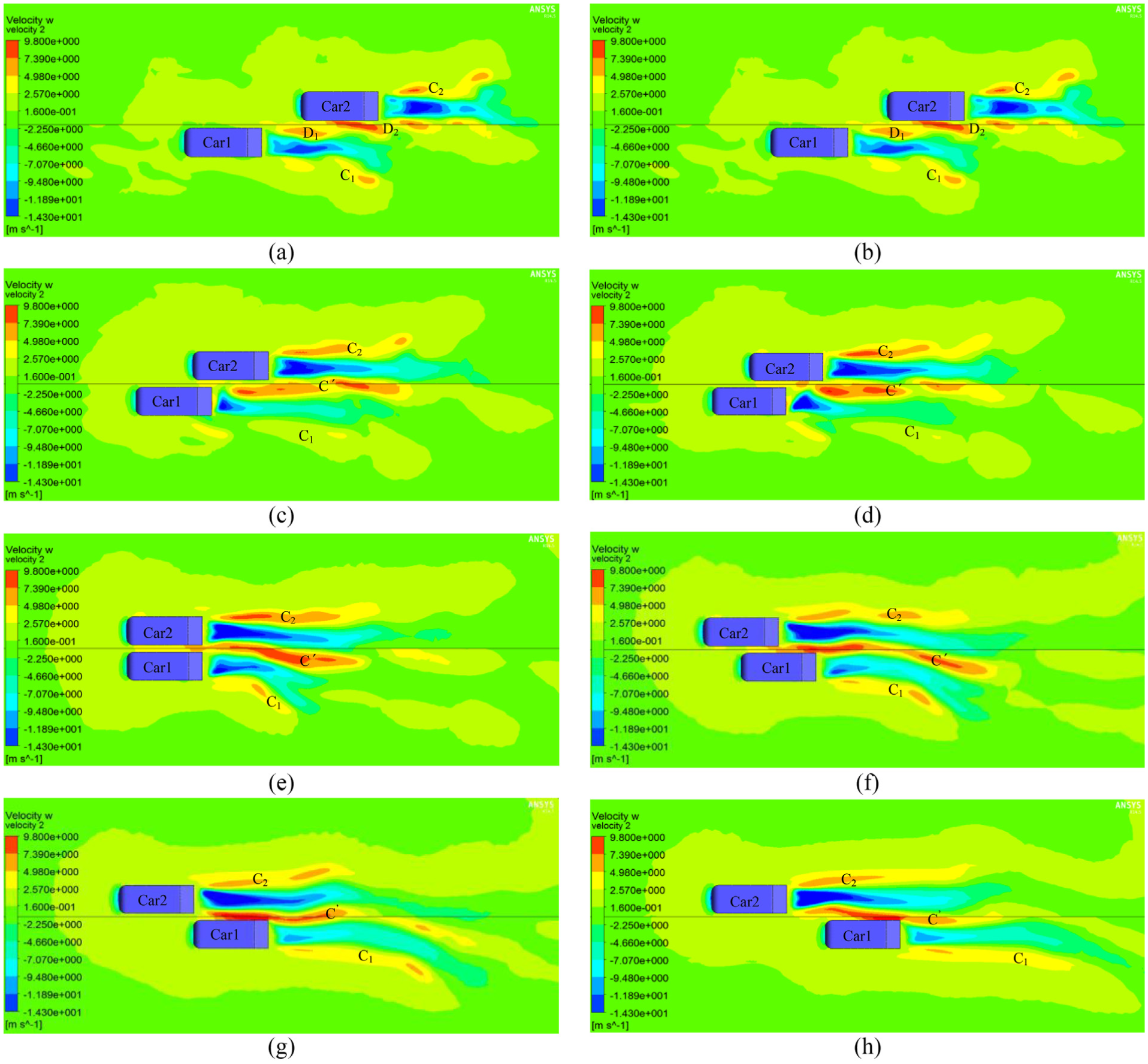
Velocity of the flow field during the overtaking maneuvers: (a) Location −1.5, (b) Location −1, (c) Location −0.75, (d) Location −0.5, (e) Location 0, (f) Location 0.5, (g) Location 1, and (h) Location 1.5.

Figure 13.

The structure of C′.

The pressure field and the vortex structure

Figure 14 shows the vortex structures and pressure fields in several specific positions during the overtaking maneuvers under the condition of V_r = 10 m/s, Y/W = 0.25. The isosurface provides the availability to clearly observe the vortices in the flow fields.

Figure 14.

The contours of the pressure and the isosurfaces of the velocity and Q criterion to extract vortices around the vehicles: (a) Location −1.5, (b) Location −1, (c) Location −0.75, (d) Location −0.5, (e) Location 0, (f) Location 0.5, (g) Location 1, and (h) Location 1.5.

It is observed from Figures 7 and 14(a) that D₁ obviously leans to the outer side of Car2 while other flows around the two vehicles have little change. When Car2 moves to Location −1, the leaning of D₁ decreases while the length of it increases. The high-pressure regions in front of the two vehicles are combined to one high-pressure region named P. The area of P decreases when Car2 moves to Location −0.75 and C′ leans to Car1 at this location. To clarify the variations in the flow fields during the overtaking maneuvers, the overlap length of the two vehicles is defined as g, as shown in Figure 14. With the movement of Car2, the area of P decreases and reaches to its minimum at Location 0. At this location, P is X-axial symmetric, and the trailing vortices of the two vehicles are also X-axial symmetric. After this location, the two vehicles start to separate. P is divided into two regions in front of the two vehicles and D₂ leans to the outer side of Car2 in the near-trail region.

The vorticity of the flow fields

The contours of vorticity on the plane across the mass center are shown in Figure 15. When the overtaking maneuvers begin, the high-vorticity regions (marked in red) of Car2 expand while the length of D₂ has little variation. However, the high-vorticity regions of Car1 have little variation while the length of D₁ remarkably decreases and leans to the outer side of Car1. With the movement of Car2, the high-vorticity regions of Car1 expand. When Car2 moves to Location −0.75, C′ comes into being. The vorticity of C′ is defined as the sum of the absolute values of the vorticities of D₁ and D₂. As two vehicles get closer, the velocities of I₁ and I₂ increase, as shown in Figure 12. I₁ and I₂ are attached flow, which means the high velocities and the low vorticities of them. When I₁ and I₂ evolve downstream, they cross C′ through the middle of it. As a result, the velocity of the middle of C′ is high while the rotating speed is low. It can be seen from Figure 15 that the vorticity of the middle region of C′ is low (marked in blue), and the vorticity of the both sides of C′ is high (marked in yellow). The vorticity of C′ is negatively correlated to the velocity of C′. Because the vorticity of C′ cannot be directly obtained from Figure 15, the vorticity of C′ is indirectly obtained from the velocity of C′. The vorticity of C′ at this position is the biggest during overtaking maneuvers.

Figure 15.

The vorticity of the turbulent flow during the overtaking maneuvers: (a) Location −1.5, (b) Location −1, (c) Location −0.75, (d) Location −0.5, (e) Location 0, (f) Location 0.5, (g) Location 1, and (h) Location 1.5.

The vortex structure of Vortices A, B, and E and the pressure coefficient of slant planes of vehicles

Figures 16 and 17 show the variations in Vortices A, B, and E of both vehicles during the overtaking maneuvers. To compare the size of the vortices, the coordinates are built in the figures. Because both Vortex B and Vortex E are formed from the separating flow along the roof, the velocities of B and E are positively correlated to each other. In the streamline figures, the density of the streamline represents the velocity of the flow. The denser the streamline, the higher the velocity.

Figure 16.

The streamline of Vortices A₁, B₁, and E₁: (a) Location −1.5, (b) Location −1, (c) Location −0.75, (d) Location −0.5, (e) Location 0, (f) Location 0.5, (g) Location 1, and (h) Location 1.5.

Figure 17.

The streamline of Vortices A₂, B₂, and E₂: (a) Location −1.5, (b) Location −1, (c) Location −0.75, (d) Location −0.5, (e) Location 0, (f) Location 0.5, (g) Location 1, and (h) Location 1.5.

Taking V_r = 10 m/s, Y/W = 0.25 as an example, when Car2 moves from Location −1.5 to −0.75, the velocities of E₁ and B₁ increase. Then, these velocities start to decrease until Location 1. After that, these velocities increase again until the end of the overtaking maneuvers. It is worth noting that there is no vortex structure on the slant after Location 0.5. Comparing this variation to Figure 18, the variation tendencies are identical.

Figure 18.

The pressure coefficient of slant planes of vehicles.

Figure 17 shows the variations in Vortices A₂, B₂, and E₂ during the overtaking maneuvers. When Car2 moves from Location −1.5 to −1, the velocities of E₂ and B₂ increase. Then, these velocities start to decrease. Until Location −0.5, these velocities increase again. When Car2 moves to Location 1, these velocities decrease again until the end of the overtaking maneuvers. It is worth noting that there is vortex structure on the slant only at Location 1.

Figure 18 shows the pressure coefficient on slant planes of vehicles in the condition of V_r = 10 m/s, Y/W = 0.25. Because the slant is on the upper rear of the vehicle, the pressure on the slant obviously influences C_pm, C_d, and C_l.

Figures 19–21 shows C_pm, C_d, and C_l during the overtaking maneuvers in the condition of V_r = 10 m/s, Y/W = 0.25, respectively. By respectively comparing Figures 18–21, C_pm is positively correlated to C_p, and C_d, C_l are negatively correlated to C_p.

Figure 19.

C_pm during the overtaking maneuvers.

Figure 20.

C_d during the overtaking maneuvers.

Figure 21.

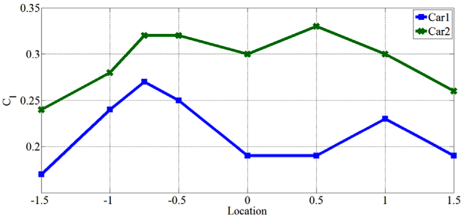
C_l during the overtaking maneuvers.

Discussion of the variations in the aerodynamical coefficients

Location −1.5

The overtaking maneuvers discussed in this article begin at this location. Car2 moves fast toward Car1 from one side, which breaks the symmetry of the initial flow fields (as Figure 7 shows) around the vehicles and causes the change in the flow fields. As a result, C_y and C_m of both cars start increasing from zero, as shown in Figure 10. Because of the influence of L₂, D₁ and C₁ are weakened (as shown in Figure 14(a)).

The fast movement of Car2 has influences on itself in two aspects. First, it strengthens Vortices C₂ and D₂ (as shown in Figure 15(a)) and generates a low-pressure region E over the slant, which decreases the pressure along the roof and the trail. As a result, C_d, C_l, and C_pm of Car2 increase. Second, it increases the velocity of the flow along the roof, which further enhances the lift force, as shown in Figure 10(d).

The movement of Car2 also influences the flow fields of Car1. As the two vehicles get closer, the influences between L₂ and D₁ increase, and the velocity and vorticity of D₁ decrease (as shown in Figures 12 and 15). Then, the unbalanced C₁ and D₁ produce different forces acting on Car1, leading to a clockwise yaw moment acting on Car1. Consequently, the two vehicles have a tendency to get closer.

Location −1

As the distance between Car1 and Car2 further decreases, the influence of the flow fields around Car2 acting on Car1 increases.

First, L₂ moves along with Car2. L₂ starts to influence L₁, and subsequently, region P is formed (as shown in Figure 14(b)). And the area of P reaches its maximum at this moment. Because of the formation of P, C_d and C_y of Car1 and C_d of Car2 sharply increase (as shown in Figure 10).

At the beginning of the overtaking maneuvers, Car2 has an anti-clockwise rotation tendency because of the attractive force generated by the interaction of L₂ and D₁. During this period, the magnitudes of C_y and C_m of Car2 are positive, and the dominant factor that influences the velocity of I₁ is L₂. Then, with the movement of Car2, I₂ and I₁ start to influence each other. Because the velocity of I₂ is higher, I₁ is accelerated, which decreases the pressure along the inner side of Car1. As a result, C_y of Car1 increases to its positive maximum (as shown in Figure 10(b)).

At the same time, due to the high pressure of L₂, the inner rear of Car1 is pushed away from Car2, resulting in a decrease in C_m of Car1, as shown in Figure 10(c).

Finally, I₂ accelerates D₁, making the pressure of the rear of Car1 further decrease and C_d of Car1 further increase to its maximum during the overtaking maneuvers. Simultaneously, the accelerated D₁ enhances Vortices B₁ and E₁ (as shown in Figure 16(b)), which accelerates the flow along the roof of Car1, making C_l of Car1 increase (as shown in Figure 10(d)). Due to the potential-flow character of D₁, the enhancement of D₁ makes a longer trailing vortex, as shown in Figure 14(b).

Before this location, these two vehicles influence each other because of the flow fields in front of Car2 acting on Car1. After this location, the wake flows of two vehicles start to influence each other.

Location −0.75

L₂ moves with Car2, reducing the influences acting on C₁ and D₁. As a result, C_m of Car1 increases. Simultaneously, the vorticity of C′ at this position is the biggest during overtaking maneuvers, as shown in Figure 15. And C′ exerts a great effect on Car2. At this position, C′ leans to Car1, trailing Car2 close to Car1, as shown in Figure 14. Consequently, C_m of Car2 reaches to its minimum, as shown in Figure 10(c). And C′ makes the pressure of E reach its minimum, as shown in Figure 18. As a result, C_pm reaches the peak during the overtaking maneuvers, as shown in Figure 10(e).

Location −0.5

The degree of the interaction between L₁ and L₂ gets higher, further slowing down the velocity of the flow in region P. Therefore, the pressure of L₁ and C_d of Car1 increases.

L₂ decreases the velocity of the flow on the inner rear of Car1, as shown in Figure 14, which increases the pressure on the inner rear of Car1 to the maximum. As a result, C_m of Car1 reaches its maximum (as shown in Figure 10(c)). Simultaneously, the velocity of I₁ and I₂ increases, as shown in Figure 12(d). Because I₁ and I₂ are mainly attached flow, the rotating speed of Vortex B of both vehicles is slowed down, as shown in Figures 16(d) and 17 (the streamline of Vortices A₂, B₂, and E₂), slowing down the velocity of the flows over the roofs of both vehicles. Consequently, C_l of both vehicles decreases.

Location 0

At this location, the two vehicles travel in parallel. As a result, the flow fields are basically symmetric and C_m of both vehicles is zero. L₁ and L₂ intensively interact with each other and make the velocity of the flow in P reach the lowest. At this location, P is X-axis symmetric while L₂ is a little larger than L₁, which makes the pressure drag of Car2 a little larger than that of Car1. Simultaneously, the inner area between Car1 and Car2 diminishes to the minimum, greatly accelerating I₁ and I₂. Then, a strong negative-pressure region is formed, dragging both vehicles to each other and taking C_y of both vehicles to the maximum. Meanwhile, the velocities of I₁ and I₂ increase to the maximum, and the rotating speed of Vortex B of both vehicles is slowed down to the minimum. Consequently, C_l of both vehicles decreases to the minimum.

Location 0.5

With the separation of the two vehicles, the interacting degree of L₁ and L₂ starts reducing and the interacting degree of L₁ and I₂ increases. That means L₁ is accelerated while I₂ is decelerated. As a result, C_d of Car1 decreases and the pressure between them increases. At this location, the tendency that the two vehicles get close to each other stops, and C_y of both vehicles decreases when C_m of Car2 decreases (clockwise). The vorticity of C′ restarts to increase, magnifying C_l of both vehicles.

Location 1

At this location, I₁ starts to accelerate D₂, magnifying C′ which drags Car2 close to Car1, as shown in Figure 14. On one hand, the circumferential velocities of Vortex B of both vehicles increase, making C_l of both vehicles reach the maximum. On the other hand, C_m of Car2 reaches the minimum (clockwise). Simultaneously, the high pressure in L₁ acts on the inner side of Car2, pushing both vehicles away from each other and making the C_y of Car2 reach the minimum.

Location 1.5

With the separation of the two vehicles, the influences of the flow fields around the two vehicles decrease. The aerodynamical coefficients of the two vehicles are gradually close to the initial values shown in Table 5.

Conclusion

In this article, the variations in the flow fields around the two vehicles during the overtaking maneuvers are discussed in detail, and the pressure, velocity, vorticity, and vortex structure of the flow fields are analyzed comprehensively. According to the study conducted in this article, the following conclusions can be drawn:

1. The pressure of E remarkably influences the lateral aerodynamical coefficients—C_pm, C_d, and C_l. C_pm is positively correlated to C_p while C_d and C_l are negatively correlated to C_p.

2. The velocities of I₁ and I₂ change dramatically during the overtaking maneuvers. On one hand, the variations in the velocities of I₁ and I₂ influence the pressure on the inner sides between the two vehicles, which influences C_y and C_m. On the other hand, when I₁ and I₂ evolve downstream, the velocity and vorticity of C′ are changed, which also influences the aerodynamical coefficients.

3. Because of the low velocity and high pressure of L, the aerodynamical coefficients of the two vehicles are influenced by the variations in locations of L.

4. The variations in V_r cause the variations in the velocities of all the flow fields, influencing the aerodynamical coefficients.

5. When V_r is constant, the variation in Y/W mainly influences the velocities of I₁ and I₂, which influences not only the pressure on the inner sides between the vehicles but also the velocities and vorticities of trailing vortices.