Sage Journals: Discover world-class research

Abstract

Health monitoring of train bearing is crucial to railway transport safety. More and more attention has elicited by the wayside acoustic monitoring technique in recent years than other defect detection techniques. However, wayside acoustic signal contains serious Doppler distortion and heavy background noise because of the high speed of trains. Thus, extracting fault-relevant information is difficult. A novel method for Doppler effect correction is proposed in this study by incorporating the traditional time-domain interpolation resampling with a novel kinematic parameters estimation method. In this kinematic parameters estimation method, an iterative algorithm based on least squares theory is proposed to improve the parameters estimation accuracy. After the Doppler effect correction, the ensemble empirical mode decomposition is employed to further enhance the fault-relevant information. The proposed iteration algorithm can improve the accuracy of kinematic parameters estimation significantly; thus the Doppler distortion can be corrected more accurately. The proposed ensemble empirical mode decomposition can further enhance the fault-relevant information and so that the accuracy and reliability of the diagnosis decision can be improved. The performance of this method has been verified in experimental and simulated cases.

Keywords

Train bearing fault diagnosis wayside acoustic monitoring kinematic parameters estimation ensemble empirical mode decomposition

Introduction

Railway transport is one of the main transportation modes for national economic activities and general public travel. The safety, stability, effectiveness, and economy of railway transport are current concerns. Bearings are critical components in train wheels. If a bearing fault cannot be determined in time, a serious accident could occur. Therefore, monitoring the status of the train wheel bearing is necessary to prevent railway traffic accidents and reduce economic losses and casualties.^1,2

Train bearing fault diagnosis can be performed through several methods, such as oil monitoring,³ hot-box detection,⁴ vibration signal analysis,⁵ and acoustic signal analysis.⁶ Wayside acoustic signal (WAS) diagnosis has a clear advantage over other methods because the acoustic signal acquisition device does not come into contact with the wheel bearings. As a train passes over a track, the WAS of wheel bearings can be obtained with a wayside microphone mounted next to the track. When the wheel bearing is faulty, fault-induced impulses exist in the acquired signal. Many mechanical faults can be detected from wheel bearing signals. The signal acquisition system of the acoustic analysis method is also simple and economical. This technique can predict incipient failures and conduct on-line monitoring.⁶

However, given the relatively high moving speed between the microphone and the train, the Doppler effect will make the WAS a serious distortion.⁷ Consequently, the signals undergo amplitude modulation and frequency band expansion. The collected WAS are also submerged in heavy noises, such as rolling noise,⁸ mechanical structural borne noise radiated by car body vibration,⁹ and aerodynamic noise.¹⁰ In addition, many frequency interference components also exist in the WAS because of adjacent wheel bearing. These problems make extracting fault information from WAS difficult. Thus, the accuracy, validity, and stability of the method are affected.¹¹

In order to correct the Doppler effect using time-domain interpolation resampling (TIR) method, the kinematic parameters of the WAS must be identified. There are two ways to do it at present: one is kinematic parameters estimation (KPE) based on the data-driven matching pursuit method, and the other is KPE based on the instantaneous frequency (IF) extraction.¹² However, the algorithm of data-driven matching pursuit method usually takes a long time, and with the increase in the number of kinematic parameters, the required time will grow very fast.¹³ The accuracy of KPE based on the IF extraction is generally low and should be improved further.¹⁴ In addition, a narrow fitting interval should be set for each parameter beforehand in traditional method. This condition limits the traditional method because the fitting intervals for each parameter cannot be set in each fitting, due to several parameters that are unknown in advance. Thus, in this study, an iterative fitting algorithm that involves the iterative extraction of IF through iterative kinematic parameter fitting is proposed to improve the accuracy of KPE. Through iterative fitting, the accuracy of the obtained kinematic parameters increases until the optimal value is reached. The optimal kinematic parameters will be used to correct the Doppler effect of the WAS according to TIR.^15,16 In TIR, the higher the accuracy of the obtained kinematic parameters is, the better the results of acoustic signal correction are. Thus, this study focuses on improving the accuracy of the obtained kinematic parameters.

Even after correcting the Doppler effect, identifying the fault information of the wheel bearing remains difficult because of the heavy background noise. The next task is to extract weak fault-relevant information (FRI) from WAS with heavy background noise. Many methods have been developed in recent years to enhance the FRI of rotating machinery. These methods include digital filters,¹⁷ wavelet transform,^18,19 stochastic resonance,^20–22 manifold learning,²³ match pursuit,²⁴ and morphological analysis.²⁵ Empirical mode decomposition (EMD) is a classical method that could be used to extract the time–frequency feature of non-stationary and non-linear signals.^26–28 The mode-mixing problem of EMD can be eliminated by ensemble empirical mode decomposition (EEMD),^29,30 which is a noise-assisted method. In this study, the Doppler-free signal is first decomposed into a set of embedded natural oscillatory modes by EEMD; those modes are defined as intrinsic mode functions (IMFs).³¹ Second, spectral kurtosis is calculated to select the IMF that represents the failure characteristic. Finally, the local fault frequency of the WAS can be identified by envelope spectrum analysis on the chosen IMF.

The contents of this article are arranged as follows: the research background, which includes the kinematic model, and theory of TIR is introduced in section “Research background.” Section “Proposed fault diagnosis strategy” introduces the iterative fitting algorithm of KPE, which is the core of the WAS monitoring technique. Section “Simulation analysis” presents the results of the simulation process to verify the effectiveness of the iterative fitting algorithm. Section “Experiment analysis” discusses the results of the experimental test using bearings with outer and inner race defects, and the result of the experiment verified the performance of the proposed method in WAS diagnosis. Section “Conclusion” presents the conclusions of the study.¹

Research background

Kinematic model

The kinematic model is shown in Figure 1. When a train passes over a track in reality, the WAS generated by the train wheel bearings are collected by the microphone installed at the wayside. The distance between the train and microphone varies, and the train speed is high. Thus, the WAS obtained from the wayside contains serious frequency distortion caused by Doppler effect. In Figure 1, v is the train speed, s is half the track length, the distance between the microphone and wheel bearing is represented by R, and the vertical distance between the microphone and wheel bearing is represented by r. Given the train movement, R shortens from a point to the midpoint of the track (O) and then lengthens after the train passes over the midpoint (O). f₀ is the center frequency of the acoustic signal. It should be time-varying and can be denoted by f₀(t). The kinematic model is described as equation (1)

γ = {f_{0}, v, r, s}

(1)

Figure 1.

Kinematic model of a train.

The time-varying center frequency f₀(t) can be expressed as equation (2) according to the theory of dynamics and the kinematic model, where M is the Mach number in aerodynamics³² defined as M = v/c, and c is the speed of sound spread in the air (i.e. generally, c is 340 m/s). After simplification, the Doppler frequency time-varying formula can also be expressed as equation (3). The proposed iterative fitting algorithm is implemented according to the following two frequency formulas

f_{0} (t) = f_{0} \cdot \frac{M (s - vt) + \sqrt{{(s - vt)}^{2} + (1 - M^{2}) r^{2}}}{(1 - M^{2}) \sqrt{{(s - vt)}^{2} + (1 - M^{2}) r^{2}}}

(2)

f_{0} (t) = \frac{1}{1 - M \cos θ} \cdot f_{0}

(3)

Doppler correction using TIR

TIR can provide a good result of Doppler distortion correction both in single- and multiple-frequency Doppler distortion signals. The amplitude and frequency structures of the distortion signal can be both corrected by TIR.

The following is a brief introduction of the TIR algorithm principle. The TIR framework is depicted in Figure 2, and the steps of the TIR method are described as follows:

First, the optimal kinematic parameters are used to calculate the resampling time vector ${t_{R}}$ and amplitude demodulation factor ${A_{d}}$ .

Second, the Doppler distorted signal ${x (t)}$ is demodulated by amplitude demodulation factor ${A_{d}}$ into a demodulated signal ${x_{d} (t)}$ , where ${x_{d} (t)} = {x (t)} * {A_{d}}$ .

Third, ${t_{R}}$ is then applied to resample the demodulated signal ${x_{d} (t)}$ for the Doppler-corrected signal ${x_{d} (t_{R})}$ . A detailed introduction of this algorithm is presented in the study of Liu et al.¹⁵

Figure 2.

TIR flowchart.

Proposed fault diagnosis strategy

After pre-processing of the input signal, the main task of this method is to estimate the kinematic parameters. This method obtains the iterative kinematic parameters by fitting the iterative IF. The optimal kinematic parameters can be obtained by fitting the most accurate IF based on least squares theory according to equation (2). The most accurate IF can be extracted from the iterating kinematic parameters by setting a threshold beforehand. The optimal kinematic parameters will be used to correct the distorted signal according to TIR; then, the fault information will be identified by EEMD. The flowchart of this method is shown in Figure 3, and its detailed description is as follows:

The original signal X(t) has serious Doppler distortion and is mixed with heavy noise and interference from different sound sources.

Signal pre-processing—the signals with the frequency of interest from the original signals can be obtained through a Butterworth band-pass filter with a specific frequency band. The time–frequency distribution (TFD) of X(t) is obtained by time–frequency analysis.^33–35 It uses short-time Fourier transform (STFT) in this study. The time–frequency matrix TF(t,f) of X(t) is constructed from TFD. An energy threshold of time–frequency matrix TF(t,f) is set to reduce the background noise and interference components with a mean filter.^36,37 The energy threshold is defined as $E = \sum_{i = 1}^{n} \sum_{j = 1}^{m} {TF}_{(t_{i}, f_{j})}^{2} / (n * m)$ , where n is the length of column of matrix TF(t,f), m is the length of rows of matrix TF(t,f). The signal is expressed as x(t) after pre-processing.

IF ridge line extraction—the IF ridge line can be extracted by connecting the energy extreme points. From TFD of x(t), IF should be located where the high energy is, where the IF could be defined as ${f_{0} (t), t = 1 \dots N}$ .

First KPE—the kinematic parameters (i.e. f₀, v, r, and s) are estimated by curve fitting the IF ridge line extracted in step 3 with equation (2).

Kinematic parameter computation—the kinematic parameters are calculated according to the Doppler frequency variation formula (3). The first point of the IF extracted by step 3 is selected for computation because it is the simplest case. The IF is shown in formula (2). At this point, t = 1, f_e is the emitting frequency expressed by $f_{e} = \sum_{1}^{N} f_{0} (t) / N$ , the receiving frequency is expressed by f_r = f₀ (t = 1), and cosθ can be expressed as $\cos θ = vt / \sqrt{v^{2} t^{2} + r^{2}}$ . Thus, equation (3) can further evolve into equation (4)

\frac{v^{4} \cdot t^{2}}{v^{2} t^{2} + r^{2}} = {(c - \frac{c f_{e}}{f_{r}})}^{2}

(4)

where $(c - c f_{e} / f_{r})^{2}$ is written as a. Through the first KPE, the f_r and f_e values are not only already known but also they are also almost accurate, although the fitting of the other parameters produces a large deviation. c is the speed of sound in air, so a is a constant. The aforementioned formula can be simplified as equation (5)

\frac{v^{4} \cdot t^{2}}{v^{2} t^{2} + r^{2}} = a

(5)

where t is half of the length of the sample time series. Once the sound acquisition device is installed, r becomes constant. Thus, the train speed v can be solved through equation (5). Given that the train speed v and time t(i) is known, the horizontal distance can be obtained as equation (6)

s = v \cdot t

(6)

Doppler window construction—a set of highly accurate kinematic parameters (i.e. v, s, r, and f₀) are obtained after step 5. The time series t(i) with the length of the signal generates a time–frequency curve with Doppler distortion in TFD according to equation (2). The Doppler windows are constructed with upper and lower boundaries. The boundaries of the Doppler window can be expressed as: (1 ± k*rf)·f₀(t). The distance between upper boundary and the time–frequency curve is defined as range factor rf. The initial value of rf is 0.01. The value of k is generally defined as $k = \max [f_{0} (t)] / (\max [f_{0} (t)] - \min [f_{0} (t)])$ .

Iterative termination judgment—rf is set as the iteration termination condition. If the condition is satisfied, the iteration will be terminated, and the output would be the optimal value. Otherwise, the process will return to step 3, and the IF ridge line will be extracted again. A new Doppler window with a reduced width is then constructed, where the width of the each reduction is 0.002 and the window width threshold is set as 0.001. In each iteration, a set of new parameters can be obtained, and the Doppler window can be constructed again based on this set. When searching for the extreme value of energy of each column in the Doppler window, IF can be obtained by connecting each extreme value. The accuracy of the obtained IF and kinematic parameters is then improved.

The obtained kinematic parameters are employed by TIR to correct the Doppler effect.

EEMD is adopted to decompose the corrected signal into a set of IMFs. One of the IMFs is selected as the diagnosis information based on the spectral kurtosis maximum principle.

Fault frequency is identified through envelope spectrum analysis.

Figure 3.

Flow diagram of the WAS diagnosis method.

Simulation analysis

A simulation signal was designed to verify the proposed method. The kinematic parameters were designed as follows: s = 1.5 m, r = 1 m, v = 45 m/s, and c = 340 m/s. The simulated Doppler-shifted signal can be expressed as equation (7)

x (t) = \sum_{i = 1}^{4} \frac{2 π P_{i} f_{i}}{4 π R {(1 - M \cos θ)}^{2}} \cos (2 π f_{i} (t - \frac{R}{c}))

(7)

where the intensities of four frequency components are as follows: P₁ = 0.7, P₂ = 1.7, P₃ = 0.9, and P₄ = 1.1. f_i is defined as the center frequency of the simulated distortion signal, and the simulated Doppler signal comprises four frequency components (i.e. f₁ = 1000 Hz, f₂ = 1300 Hz, f₃ = 1500 Hz, and f₄ = 1700 Hz). The sampling frequency in this simulation was 50 kHz. Considering the actual scenario where the acoustic signal contains heavy noises, a random noise n(t) was added to the simulation signal, where $n (t) = D \cdot ξ (t)$ ; $ξ (t)$ express the random noise with zero mean, D is the deviation of the noise, where D = 7. The final simulation signal is described as equation (8). The simulative Doppler distortion signal is displayed in Figure 4(a). The spectrum of the simulation signal is displayed in Figure 4(b)

x_{s} (t) = x (t) + n (t)

(8)

Figure 4.

(a) Simulative Doppler distortion signal and (b) spectrum.

Given that all frequency components follow the same distortion rule, one of the frequency components, that is, f₂ = 1300 Hz, was selected to iterative IF extraction and curve fitting, in order to get the optimal kinematic parameters of the simulation signal. The simulation signal was pre-processed by a filter, and energy threshold was set to eliminate the background noise and interference components. Where, the energy threshold of simulation signal is 200.88 (in TFD). The processing of the iterative fitting algorithm is shown in Figure 5. The width of the Doppler window becomes increasingly narrow from Figure 5(a)–(f). Each iteration is a new process of IF extraction and parameters fitting, and the new kinematic parameters become increasingly accurate until a set of optimal values is obtained. The values of the kinematic parameters obtained in the first fitting were compared with the optimal values obtained by iterative fitting in Table 1. The improvement in the accuracy of the kinematic parameters is evident. The receive time vector ${t_{R}}$ and amplitude demodulation factor ${A_{d}}$ can be calculated according to TIR based on the optimal kinematic parameters. ${A_{d}}$ is shown in Figure 6(a), and ${t_{R}}$ is shown in Figure 6(b). The Doppler distortion contained in the acoustic signal is almost completely removed, and the result can be seen in Figure 6(c).

Figure 5.

Iterative process demonstration with the simulation signal: (a) the renderings of first iteration, (b) the renderings of second iteration, (c) the renderings of third iteration, (d) the renderings of fourth iteration, (e) the renderings of fifth iteration, and (f) the renderings of sixth iteration.

Table 1.

Different fitting results of simulation signal.

Parameters	f ₀	v	s	r
Actual value	1300 Hz	45 m/s	1.5 m	1 m
First fit value	1283.10 Hz	40.25 m/s	1.20 m	0.79 m
Error (%)	1.30	10.56	20.00	21.00
Optimal value	1288.40 Hz	44.90 m/s	1.45 m	1.12 m
Error (%)	0.89	0.22	3.33	12.00

Figure 6.

(a) Amplitude demodulation factor, (b) resampling time series, and (c) TFD of Doppler-free signal.

Experiment analysis

Experiment setup and data acquisition

The experiment was divided into two separate steps. The microphone collects the acoustic signal of the faulty bearing from the bearing test workbench in the first step. A kinematics experiment that allowed the fault acoustic signal to generate Doppler distortion was conducted in the second step. The outer and inner race faults of the bearing were tested in the experiment. Figure 7 shows cracks on the outer and inner races, which were cut by a wire-electrode cutting machine. The width of the cracks all set as 0.18 mm.

Figure 7.

Bearing with artificial defects: (a) artificial crack on outer race and (b) artificial crack on inner race.

The acoustic signal with the fault-induced impulses was collected by a microphone. The bearing test bench setup is shown in Figure 8(a). The bearing test workbench was composed of a drive motor, a tested bearing, and a mechanical radial loader. The microphone was installed next to the workbench.

Figure 8.

Experimental setup: (a) bearing signal acquisition system and (b) the scene of Doppler signal acquisition experiment.

The acoustic signal obtained in the first step was played by a loud speaker on the minibus to simulate the relative motion between the train and microphone. The kinematic parameters in the second step were as follows: s = 4 m, r = 2 m, and v = 30 m/s. The experiment setup is shown in Figure 8(b). The acoustic signal was collected by microphone again, and then, the obtained signal will be mixed with Doppler effect. The sampling frequencies were all set to 50 kHz in the two experimental steps. The type of bearing used in this experiment is NJ(P)3226X1. The type of microphone is 4944-A (B&K Company). The frequency range of this microphone is 16–70,000 Hz. The fault frequency from outer race and the inner race are 137 and 195 Hz.

Outer race fault signal analysis

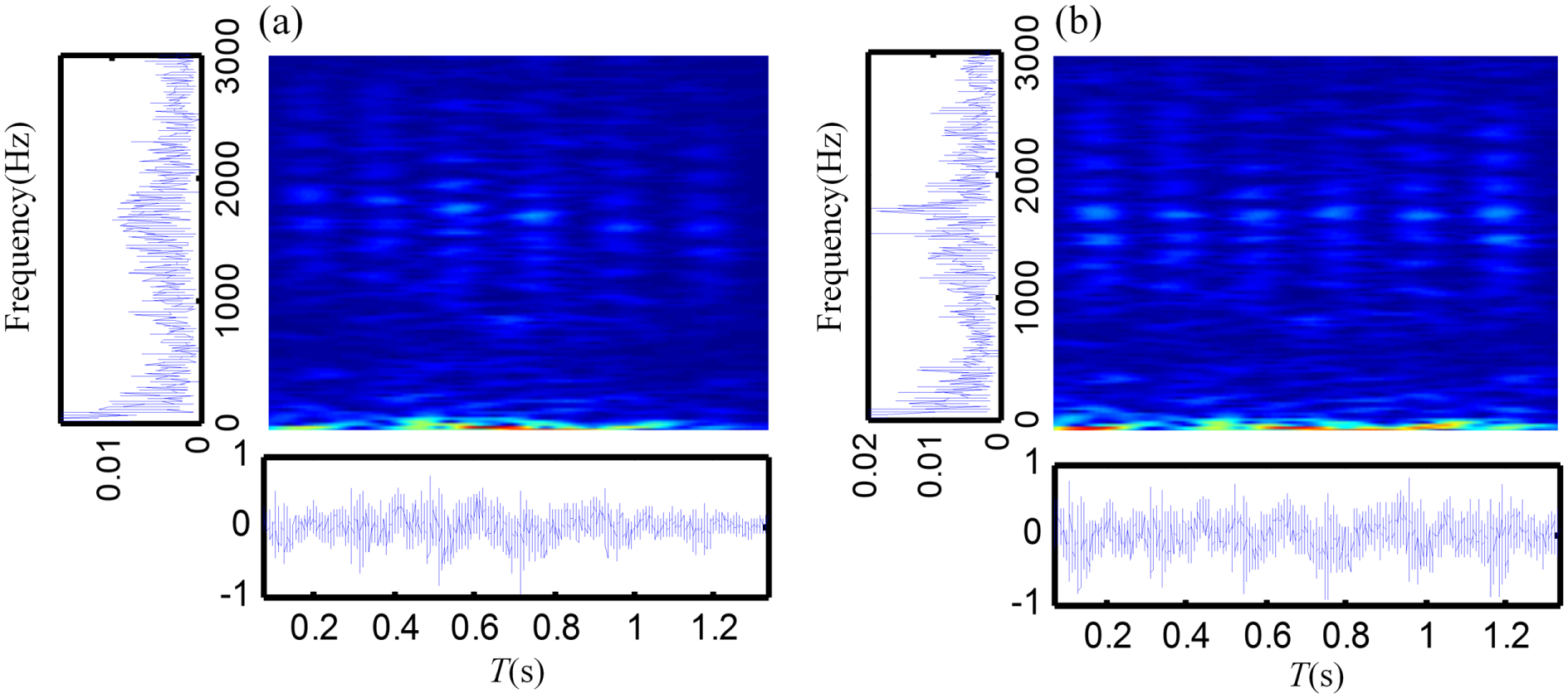
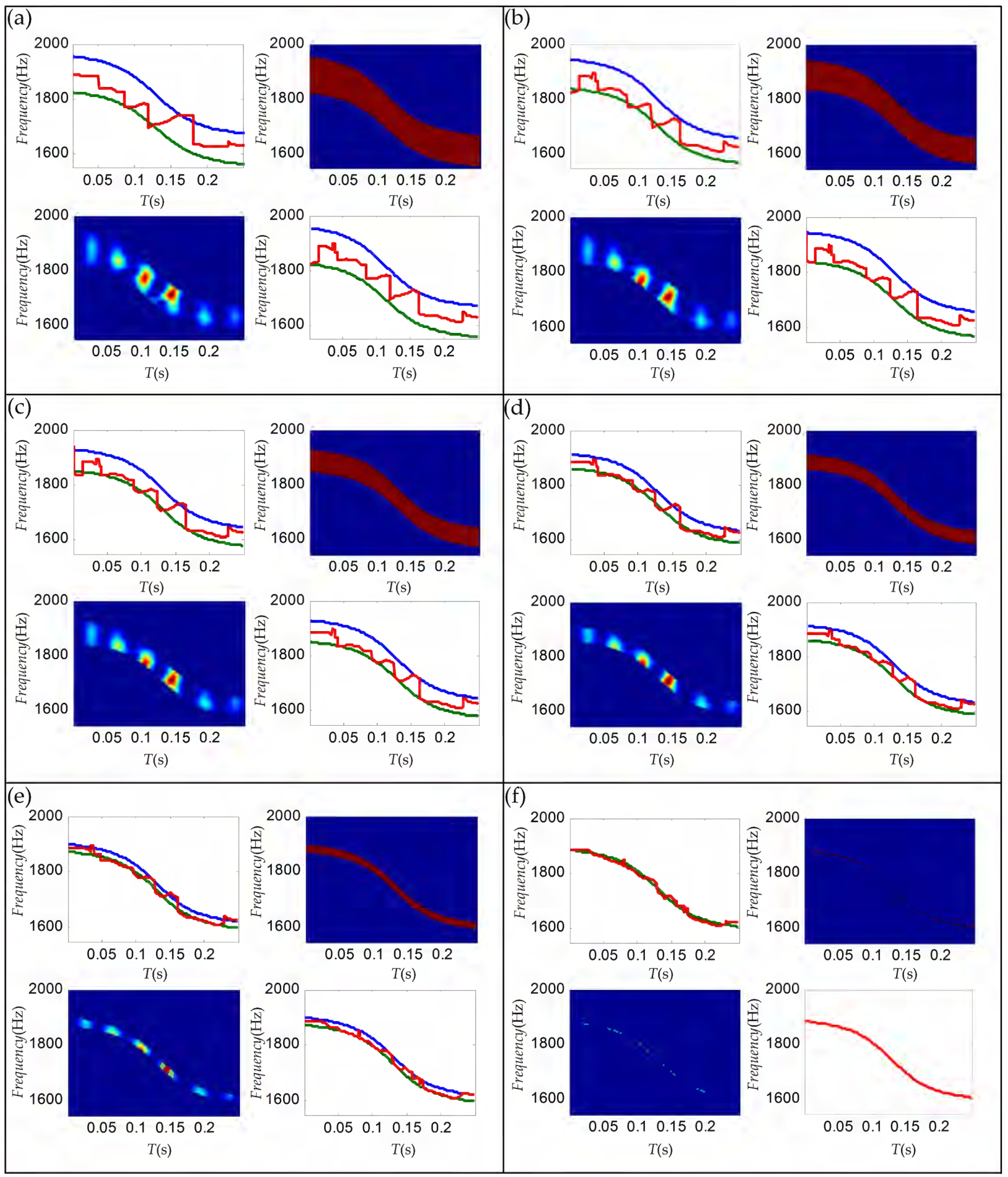
The time domain, frequency domain, and STFT of the outer race fault signal are shown in Figure 9(a). Frequency band expansion clearly existed in the frequency domain, which made the identification of the fault frequency difficult. Thus, investigating the kinematic parameters is necessary to correct the Doppler effect from the signals. The outer race signal was pre-processed by a band-pass filter with the pass-band of 1580 and 1950 Hz, and the background noise and interference components were eliminated with the energy threshold, which is 0.005 (in TFD). The KPE processing by iterative Doppler construction and curve fitting is shown in Figure 10. The width of the Doppler window becomes increasingly narrow from Figure 10(a)–(f), where the window width threshold was set to 0.001. The iterative fitting algorithm was run until rf obtained the threshold set in advance. Figure 10(f) shows that the Doppler window region approximates one curve, and the region is focused on areas with the highest signal energy. The said figure also shows that the interferences caused by other frequency components were effectively eliminated by the proposed method. The values of the kinematic parameters obtained by first fitting were then compared with the optimal values obtained by iterative fitting in Table 2. The accuracy of the kinematic parameters clearly improved because of the iterative algorithm. The Doppler effect can be corrected in the acoustic signals according to TIR and the optimal kinematic parameters. Figure 9(b) shows the time domain, frequency domain, and STFT of the correction acoustic signal. Frequency band expansion in the frequency domain was eliminated, and the signal obtained suitable correction in TFD.

Figure 9.

(a) Original signal and (b) Doppler-free signal.

Figure 10.

Iterative process demonstration with the outer race signal: (a) the renderings of first iteration, (b) the renderings of second iteration, (c) the renderings of third iteration, (d) the renderings of fourth iteration, (e) the renderings of fifth iteration, and (f) the renderings of sixth iteration.

Table 2.

Different fitting results of the outer race fault signal.

Parameters	f ₀	v	s	r
Actual value	1800 Hz	30 m/s	4 m	2 m
First fit value	1804.20 Hz	29.73 m/s	3.66 m	2.01 m
Error (%)	0.23	0.87	8.50	0.50
Optimal value	1796.83 Hz	30.14 m/s	3.91 m	2.01 m
Error (%)	0.18	0.47	2.35	0.50

After the Doppler effect was corrected, the fault information was still submerged in heavy noises. Thus, the next step was to extract weak information through EEMD. First, the Doppler-free signal was decomposed into a set of IMFs. Second, spectral kurtosis of each IMF was calculated as an index to extract fault information, as shown in Figure 11(a). The larger the spectral kurtosis of IMF is, the more fault information the IMF contains.^38,39 And it can be seen from Figure 11(a) that the third IMF value is the largest, so the third IMF was selected for the envelope spectrum analysis, where the three IMFs whose spectral kurtosis were bigger were displayed in Figure 11(b), and Figure 12(a) shows the envelope spectrum of the Doppler-free signal. Figure 12(b) shows the envelope spectrum of the third IMF. It can be seen that the fault frequency is clearer in Figure 12(b), which means that the signal was effectively de-noised.

Figure 11.

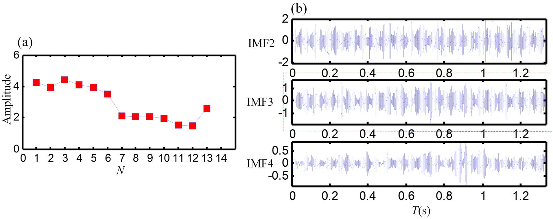
(a) Spectral kurtosis values of each IMF and (b) Second, third, and fourth IMFs.

Figure 12.

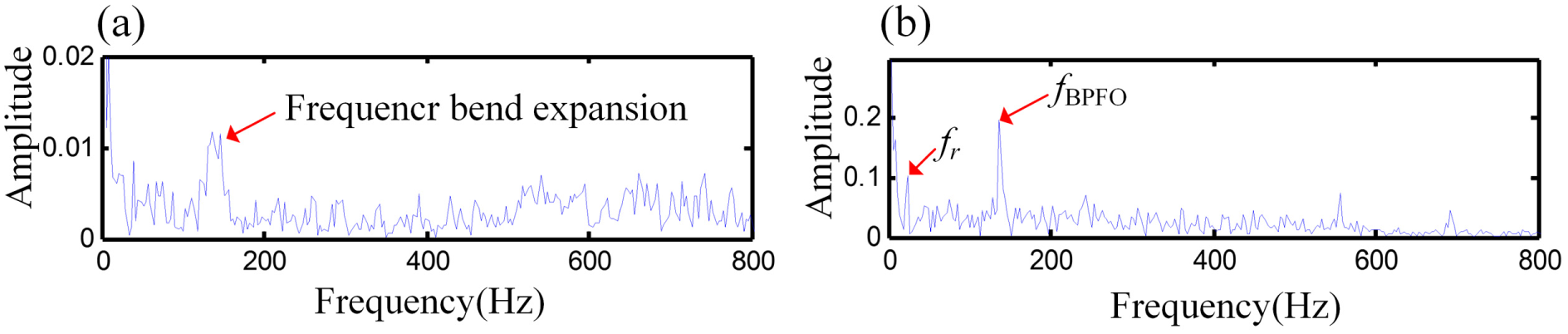
(a) Envelope spectrum of the Doppler-free signal and (b) envelope spectrum of IMF3.

Inner race fault signal analysis

The proposed WAS diagnosis method also can identify the fault information from inner race signal. The time domain, frequency domain, and STFT of the inner race signal are shown in Figure 13(a). Given the Doppler effect, the inner race fault signal also exhibits obvious frequency band expansion in the spectrum. In addition, different from the outer race signal, the TFD shows that the time–frequency region of the inner race signal is discontinuous. So, its KPE is more difficult than that of the outer race signal. After signal pre-processing with a band-pass filter of 1680 and 1950 Hz, set an energy threshold to reduce the background noise, where the calculate result of energy threshold of inner race is also 0.005 (in TFD). The iterative algorithm method was employed to analyze this signal, as shown in Figure 14(a)–(f). The Doppler window also became increasingly narrow, where the window width threshold was also set to 0.001. The iterative fitting algorithm continued until rf achieve the threshold. Interference can be eliminated easily because the Doppler window width became increasingly narrow through the iterative processing.

Figure 13.

(a) Original signal and (b) Doppler-free signal.

Figure 14.

Iterative process demonstration of the inner race signal: (a) the renderings of first iteration, (b) the renderings of second iteration, (c) the renderings of third iteration, (d) the renderings of fourth iteration, (e) the renderings of fifth iteration, and (f) the renderings of sixth iteration.

The two previous iterative processes of the iterative fitting are shown in Figure 15. Comparison of Figure 15(a) and (d) shows that the Doppler window width became narrow. Figure 15(a) shows two singular parts of the IF ridge line in this Doppler window. This phenomenon is caused by the interference component with high energy existing in the acoustic signal. It cannot be eliminated easily by pre-processing because the local extremum leads to a large deviation of the obtained IF ridge line. The singular part in Figure 15(a) with a gray mark converged with that in Figure 15(b) through the iterative processing. The other singular part was eliminated by a new extremum, as shown in Figure 15(b). Figure 15(c) and (d) illustrate similar scenarios. The extreme value of the effective signal, which was overwhelmed by the high-energy interference, was determined during the iterative algorithm.

Figure 15.

Demonstration of the two previous iterative processes: (a) instantaneous frequency extraction with singular part, (b) correction the singular part, (c) instantaneous frequency extraction with singular part again, and (d) correction the singular part again.

The kinematic parameter values obtained by the first fitting were then compared with the optimal values obtained by iterative fitting in Table 3. The accuracy of the kinematic parameters also improved. The Doppler effect was corrected in the acoustic signal according to TIR and based on the obtained kinematic parameters. Figure 13(b) shows the time domain, frequency domain, and STFT of the correction signal. The frequency band expansion in the frequency domain was eliminated, and the signal obtained suitable correction in the TFD.

Table 3.

Different fitting results of inner race fault signal.

Parameters	f ₀	v	s	r
Actual value	1733 Hz	30 m/s	4 m	2 m
Firs fit value	1751 Hz	27.93 m/s	3.18 m	2.01 m
Error (%)	1.03	6.91	20.29	0.50
Optimal value	1730.10 Hz	30.34 m/s	3.96 m	2.01 m
Error (%)	0.17	1.13	1.04	0.50

The fault information of the inner race Doppler-free signal was also difficult to identify because of the background noises. So, EEMD was adopted to extract weak diagnosis information. The spectral kurtosis values of each IMF are shown in Figure 16(a). The third IMF value is higher than others. It means that the third IMF contains more fault information than others. Considering that other IMFs only contained very little information about the original signal, only the IMFs from second to fourth are shown in Figure 16(b). Figure 17(a) shows the envelope spectrum of the Doppler-free signal. The envelope spectrum of third IMF is shown in Figure 17(b). The fault frequency is mixed in the background noises in Figure 17(a). Comparing Figure 17(a) and (b), the fault frequency and its harmonics can be seen clearly in the latter. It means that the fault information can be identified effectively from the inner race signal.

Figure 16.

(a) Spectral kurtosis values of each IMF and (b) Second, third, and fourth IMFs.

Figure 17.

(a) Envelope spectrum of the Doppler-free signal and (b) envelope spectrum of IMF3.

Conclusion

The proposed WAS diagnosis method can correct the Doppler effect first and then to identify the fault frequency effectively. The main innovation of the proposed method is the iterative fitting algorithm of KPE. The experiment analysis showed that the accuracy of the obtained kinematic parameters significantly improved with the iterative fitting, and the iterative fitting algorithm did not have to set a narrow fitting interval for each parameter beforehand. Doppler distortion was corrected effectively by TIR after obtaining the kinematic parameters. EEMD could extract the information from background noise. The fault frequency could be identified by envelope analysis on IMF. The proposed method may be applied to practical train bearing healthy monitoring systems to enhance their monitoring performance. However, the proposed method still has shortcomings. For example, the distance between the microphone and the middle of the track (r) should be constant in the iterative fitting algorithm to decrease the number of the unknown kinematic parameters. Furthermore, train speed increases in reality, so the distortion of the acoustic signal becomes increasingly serious. More interference could also occur from the different wheel bearings, so IF extraction becomes difficult. These problems should be addressed in future studies.

Footnotes

Handling Editor: Mario L Ferrari

Declaration of conflicting interests

The author(s) declared no potential conflicts of interest with respect to the research, authorship, and/or publication of this article.

Funding

The author(s) disclosed receipt of the following financial support for the research, authorship, and/or publication of this article: This work was supported by the National Natural Science Foundation of China (nos 51675001, 51505001, 51605002, and 51637001) and the Natural Science Foundation of Anhui Province (nos 1508085SQE212 and 1608085QE110). The experiment was completed in Dr Qingbo He’s laboratory in University of Science and Technology of china. The valuable and constructive comments from the reviewers to further improve this paper are sincerely appreciated.

References

Liu

Shen

et al . Doppler effect reduction scheme via acceleration-based Dopplerlet transform and resampling method for the wayside acoustic defective bearing detector system. ARCHIVE P I Mech Eng C-J Mec 2014; 228: 3356–3373.

Wang

Kong

. A new synthetic detection technique for trackside acoustic identification of railroad roller bearing defects. Appl Acoust 2014; 85: 69–81.

Wang

Fingas

. Differentiation of the source of spilled oil and monitoring of the oil weathering process using gas chromatography-mass spectrometry. J Chromatogr A 1995; 712: 321–343.

Schöbel

Pisek

Karner

et al . Hot box detection systems: as a part of automated train observation in Austria. In: Proceedings of the EURNEX–ZEL, Zilina, 30–31 May 2006, pp.157–161. Berlin: EURNEX.

Sohn

Farrar

. Damage diagnosis using time series analysis of vibration signals. Smart Mater Struct 2001; 10: 446–451.

Wang

et al . Wayside acoustic diagnosis of defective train bearings based on signal resampling and information enhancement. J Sound Vib 2013; 332: 5635–5649.

Ouyang

Zhang

et al . Online Doppler effect elimination based on unequal time interval sampling for wayside acoustic bearing fault detecting system. Sensors 2015; 15: 21075–21098.

Remington

. Wheel/rail rolling noise, I: theoretical analysis. J Acoust Soc Am 1987; 81: 1805–1823.

Kim

Hong

Song

et al . Interior noise analysis of a construction equipment cabin based on airborne and structure-borne noise predictions. J Mech Sci Technol 2012; 26: 1003–1009.

10.

Zhou

Wang

. Prediction and reduction of aerodynamic noise of the multiblade centrifugal fan. Adv Mech Eng. Epub ahead of print 12 February 2015. DOI: 10.1155/2014/712421.

11.

Dybala

Radkowski

. Reduction of Doppler effect for the needs of wayside condition monitoring system of railway vehicles. Mech Syst Signal Pr 2013; 38: 125–136.

12.

Wang

Chen

Cai

et al . Matching demodulation transform and synchrosqueezing in time-frequency analysis. IEEE T Signal Proces 2014; 62: 69–84.

13.

Liu

Shen

et al . Wayside bearing fault diagnosis based on a data-driven Doppler effect eliminator and transient model analysis. Sensors 2014; 14: 8096–8125.

14.

Zhang

et al . Doppler shift removal based on instantaneous frequency estimation for wayside fault diagnosis of train bearings. J Vib Acoust 2014; 136: 858–862.

15.

Liu

Kong

et al . Doppler effect reduction based on time-domain interpolation resampling for wayside acoustic defective bearing detector system. Mech Syst Signal Pr 2014; 46: 253–271.

16.

Wung

Wada

Juang

et al . Inter-channel decorrelation by resampling via time-domain interpolation filters derived from the time-shifting property. In: Proceedings of the IWAENC 2012 international workshop on acoustic signal enhancement, Aachen, 4–6 September 2012. New York: IEEE.

17.

Pitas

Venetsanopoulos

. Adaptive nonlinear filters. US: Springer, 1990, pp.267–311.

18.

Daubechies

. The wavelet transform, time-frequency localization and signal analysis. IEEE T Inform Theory 1990; 36: 961–1005.

19.

Han

Wang

Cai

. Background subtraction based on three-dimensional discrete wavelet transform. Sensors 2016; 16: 456.

20.

Yuan

et al . Online fault diagnosis of motor bearing via stochastic-resonance-based adaptive filter in an embedded system. IEEE T Syst Man Cyb 2016; 47: 1111–1122.

21.

Qin

Tao

et al . Adaptive bistable stochastic resonance and its application in mechanical fault feature extraction. J Sound Vib 2014; 333: 7386–7400.

22.

Wang

. Effects of multiscale noise tuning on stochastic resonance for weak signal detection. Digit Signal Process 2012; 22: 614–621.

23.

Maronna

. Alan Julian Izenman (2008): modern multivariate statistical techniques: regression, classification and manifold learning. Int Stat Rev 2011; 52: 733–734.

24.

Cui

Wang

Lee

. Matching pursuit of an adaptive impulse dictionary for bearing fault diagnosis. J Sound Vib 2014; 333: 2840–2862.

25.

Shen

Kong

et al . A fast and adaptive varying-scale morphological analysis method for rolling element bearing fault diagnosis. ARCHIVE P I Mech Eng C-J Mec 2013; 227: 1362–1370.

26.

Lei

Lin

et al . A review on empirical mode decomposition in fault diagnosis of rotating machinery. Mech Syst Signal Pr 2013; 35: 108–126.

27.

Yan

Gao

. Rotary machine health diagnosis based on empirical mode decomposition. J Vib Acoust 2008; 130: 111–120.

28.

Qin

. East implementation of orthogonal empirical mode decomposition and its application into harmonic detection. Chin J Mech Eng 2008; 21: 93–98.

29.

Huang

. Ensemble empirical mode decomposition: a noise-assisted data analysis method. Adv Adapt Data Anal 2011; 1: 1–41.

30.

Zhang

Yan

Gao

et al . Performance enhancement of ensemble empirical mode decomposition. Mech Syst Signal Pr 2010; 24: 2104–2123.

31.

Rai

Mohanty

. Bearing fault diagnosis using FFT of intrinsic mode functions in Hilbert–Huang transform. Mech Syst Signal Pr 2007; 21: 2607–2615.

32.

Liu

Wang

Guo

et al . Effects of inflow mach number and step height on supersonic flows over a backward-facing step. Adv Mech Eng. Epub ahead of print 26 January. DOI: 10.1155/2013/147916.

33.

Shi

Liang

Necsulescu

et al . Generalized stepwise demodulation transform and synchrosqueezing for time–frequency analysis and bearing fault diagnosis. J Sound Vib 2016; 368: 202–222.

34.

Feng

Chu

Zuo

. Time–frequency analysis of time-varying modulated signals based on improved energy separation by iterative generalized demodulation. J Sound Vib 2011; 330: 1225–1243.

35.

Feng

Liang

Chu

. Recent advances in time–frequency analysis methods for machinery fault diagnosis: a review with application examples. Mech Syst Signal Pr 2013; 38: 165–205.

36.

Church

Chen

Rice

(eds). A spatial median filter for noise removal in digital images. In: Proceedings of the Southeastcon, Huntsville, AL, 3–6 April 2008. New York: IEEE.

37.

Patidar

Gupta

Srivastava

et al . Image de-noising by various filters for different noise. Int J Comput Appl T 2010; 9: 24–28.

38.

Guo

Tse

Djordjevich

. Faulty bearing signal recovery from large noise using a hybrid method based on spectral kurtosis and ensemble empirical mode decomposition. Measurement 2012; 45: 1308–1322.

39.

Kong

Wei

Yan

et al . An estimating method for initial faulty time of rolling element bearing based on EEMD and spectral kurtosis. In: Proceedings of the 6th international congress on image and signal processing, Hangzhou, China, 16–18 December 2013. New York: IEEE.

Wayside acoustic fault diagnosis of train wheel bearing based on Doppler effect correction and fault-relevant information enhancement

Abstract

Keywords

Introduction

Research background

Kinematic model

Doppler correction using TIR

Proposed fault diagnosis strategy

Simulation analysis

Experiment analysis

Experiment setup and data acquisition

Outer race fault signal analysis

Inner race fault signal analysis

Conclusion

Footnotes

Declaration of conflicting interests

Funding

References