On the dynamic analysis of rotating shafts using nonlinear superelement and absolute nodal coordinate formulations

Abstract

In this article, a superelement formulation and a quadratic beam element based on the absolute nodal coordinate formulation are applied to the simulation of high-speed rotating structures. To this end, these formulations are briefly reviewed by highlighting their distinctive features. The performance of the studied formulations is examined using two numerical examples. The first test is a spinning beam example in which the transient response is examined. An unbalanced rotating shaft is studied in the second example, in which both transient and modal analyses are performed. The results produced using both formulations are compared against those produced in the commercial finite element software ANSYS and those available in literature. The article tests in a rotating machine dynamics context two element types which have not been formulated primarily with rotating applications in mind. This is useful in investigating the versatility of these elements.

Introduction

The analysis of rotating machinery dynamics is important in the design of many industrial applications, such as vacuum pumps, compressors, turbines and machine tool systems. The traditional approach to rotor dynamics modelling is to adopt one-dimensional (1D) models, where the shafts are modelled as beams and discs and impellers are modelled as rigid bodies. ¹ Correspondingly, the deformation of the shaft cross section is not considered in the classical 1D approach. In some applications, these assumptions may not be acceptable since the compliance of the discs and blades may affect the dynamics of the rotor. Also, the deformation of the shaft cross section may be significant, for example, in the case of tubular shafts commonly used in turbomachinery. The inclusion of shaft cross-sectional deformation and the flexibility of the discs and blades enables the description of centrifugal stiffening phenomena, where the internal tensional stresses lead to increased stiffness of the rotor. ² In addition, the thermomechanical effects might lead to residual internal stresses in the rotors that are often constructed of parts with different materials. To address these issues, several authors have proposed and utilised two-dimensional (2D) axisymmetric harmonic elements ³ or three-dimensional (3D) solid elements.^4,5 The 2D approach can describe the gyroscopic effect and the stress stiffening effect caused by the deformation of the shaft cross section or discs. The main assumption in the 2D approach is that the rotor is axisymmetric, which makes it unsuitable for analysing cases where either the rotor or the loading is asymmetric, which can occur, for example, due to blade loss or rubbing between the rotor and stator. On the other hand, the 3D solid element approach does not suffer the drawbacks encountered in 1D and 2D approaches. Nevertheless, the increase in computational effort makes it unpractical in some cases.

As an alternative, the transient analysis of high-speed rotors can be accomplished using a nonlinear finite element (FE) approach targeted for multibody applications. For example, nonlinear beam FEs^6–9 have proven to produce accurate results. However, nonlinear beam element models may also be unable to accurately describe systems with complex geometries.

To summarise, traditional 1D approaches to rotor dynamics might not be capable of reliable dynamic prediction in transient cases or situations where a nonlinear strain–displacement relation is needed. More accurate 2D or 3D formulations suffer from either the drawbacks resulting from the assumption of axisymmetry or high computational costs. It is for these reasons that many authors have utilised model reduction techniques.^10,11 One of these is the substructure method, which makes it possible to reduce an FE model by projecting it onto component modes. Originally, the substructure method (or modal reduction technique) was used to analyse linear dynamics problems such as modal analysis and time integration,^12,13 while later researchers^14,15 came to use the technique in the context of multibody dynamics.

The selection of the component modes is critical in the modal reduction procedure. An often used approach is based on the use of static constraint modes obtained by imposing displacements on the interface nodes, complemented with vibration modes with the interface clamped.^13,16 This is called the Craig–Bampton approach. Another popular method, called MacNeal’s method, uses the free-free vibration modes of the substructure complemented with attachment modes obtained via static loading on the interface. Different variations or combinations of these reduction methods have also been proposed. Cardona ¹⁷ and Wu and Tiso ¹⁸ combined Craig–Bampton modes with the floating frame concept to reduce the coordinates of flexible structure models. Géradin and Rixen ¹⁹ used MacNeal modes to simulate structures with unilateral contacts, such as leaf springs.

Assuming that elastic deformation remains small when the flexible body undergoes large reference motions, the global position of a particle can be defined as a superposition of the reference motion of a local frame and the elastic deformation with regard to that local frame. This approach is called the floating frame of reference formulation (FFRF) and is often used in practical applications when flexibility needs to be taken into account in multibody dynamics. By combining FFRF and modal reduction, Cardona and colleagues^16,17,20,21 and Bauchau and Rodriguez ²² introduced the so-called superelements. In the earlier publications,^20,21 the reference frame was attached to one node. Later, the reference frame was chosen based on the position of the interface nodes. ¹⁷ The latter approach was proven to be more accurate. Although the efficiency and accuracy of the FFRF-based superelement have been reported in many publications, the element is cumbersome to use as the equations of motion include state-dependent non-constant inertia terms, such as the mass matrix and the quadratic velocity vector. This is due to the nonlinear relationship between global and local frame coordinates. To reduce this nonlinearity, a generalised modal reduction method based on the absolute coordinate formulation (ACF) with a constant mass matrix was proposed in Pechstein et al. ²³ and Naets and Desmet ²⁴ There, FFRF-based and ACF-based superelements were compared, and it was concluded that the ACF-based element is more efficient and accurate. It was even found that in some cases, the results given by the FFRF-based superelement were not dependable.

In general, beam elements can be derived by using the elastic line concept. This allows accurate modelling of slender structures with uniform cross sections. This approach is, however, less suited for modelling complex-shaped flexible components, for example, rotors with discs or beams with varying cross-sectional properties. As an alternative to the conventional elastic line concept, Jonker and Meijaard ²⁵ described a set of deformation mode formulations for a 3D shear deformable beam element. The reduced linear model is obtained by applying the Craig–Bampton method to the FE model of the complex-shaped component. By relating the constraint modes to the deformation mode formulation, the potential energy of the nonlinear superelement can be determined. The kinetic energy can, in turn, be determined by expressing the absolute velocity vectors in a co-rotational frame. Thus, based on the combination of the model reduction technique and Jonker’s description, an efficient modelling approach allowing arbitrary reference body motions and deformations of complex-shaped flexible components can be obtained. ²⁶ In this approach, it is no longer necessary to use additional degrees of freedom (DOFs), for example, for defining the floating reference frame in FFRF or the generalised modal parameters in ACF. This feature is claimed to lead to improved numerical efficiency. The superelement has been validated with numerical examples, but the performance of this approach in applications of rotor dynamics where the gyroscopic effect plays a significant role is yet to be properly investigated.

Rotor systems can also be modelled using the absolute nodal coordinate formulation (ANCF). In the ANCF, the nodal coordinates of spatial FEs are defined using global positions and components of the nodal deformation gradients. ²⁷ Because of the linear relationship between nodal and position coordinates, the element mass matrix is constant and can be defined as in the linear FE approach. Contrary to the simple expression of inertial forces, the expression of element elastic forces is highly nonlinear and computationally demanding. However, due to the nonlinear description of strain, the nonlinear geometric stiffening terms encountered in high-speed rotors are automatically included in this formulation.

The objective of this article is to study the performance of the superelement formulation and the ANCF in the analysis of rotating structures. The article will make observations regarding the usability and accuracy of these approaches. In the next section, the Craig–Bampton approach is used to obtain the reduced matrices of the linear superelement. The nonlinear superelement is introduced in the third section by combining the constraint modes with the deformation mode formulation. The formulation of the ANCF-based beam element is reviewed in the fourth section, and in the fifth section, the behaviour of both formulations is studied in numerical tests. The first example is a spinning beam experiment, in which the transient response of the mechanical system is computed using the superelement formulation. The second example case consists of a rotor with an unbalanced rigid disc, in which the transient response and the Campbell diagram of the system are computed using both formulations.

Component modes and model reduction

This section briefly reviews the concept of modal reduction. In the FE method, the equations of motion for a rotor system can be written in matrix form as

$$\mathit{M}\stackrel{··}{\mathit{q}}+(\mathit{\Omega }\mathit{G}+\mathit{C})\stackrel{.}{\mathit{q}}+\mathit{K}\mathit{q}={\mathit{f}}_{\mathrm{ext}}$$

(1)

where M is the mass matrix, K is the stiffness matrix, G is the gyroscopic matrix, C is the damping matrix, q is the generalised coordinate vector, ${\mathit{f}}_{\mathrm{ext}}$ is the external force vector and $\mathbf{\Omega }$ is the rotational speed. According to the component mode synthesis approach, a set of component modes can be selected and used for projecting the generalised coordinate vector q into a reduced set of coordinates, as follows

$$\mathit{q}=\mathbf{\Phi }\mathbf{\xi }$$

(2)

where $\mathbf{\Phi }$ is a matrix representation of the selected modes. In modal reduction, the number of selected modes should be less than the original number of DOFs. In equation (2), $\mathbf{\xi }$ is the reduced set of coordinates, often called modal coordinates, with respect to the selected modes.

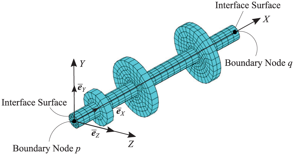
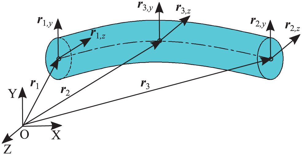
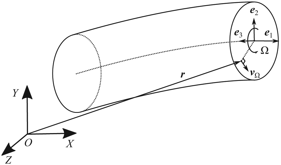
The beam-like rotor structure shown in Figure 1 is connected via two interfaces, one at each side of the component. In the case of a slender structure, such as the rotor system, the deformations of the interface can be considered to be negligible. Hence, the DOFs of the nodes on the interface surfaces can be bound with boundary nodes p and q. The deformation of the structure can be described with respect to a local reference coordinate frame attached at boundary p with unit basis $[\begin{array}{ccc}{\overline{\mathit{e}}}_X\hfill & {\overline{\mathit{e}}}_Y\hfill & {\overline{\mathit{e}}}_Z\hfill \end{array}]$ . Each boundary node has three translational $(\overline{\mathit{u}})$ and three rotational $(\overline{\mathbf{\varphi }})$ DOFs. Using the Craig–Bampton method, the FE model can be reduced with 12 static constraints plus a set of fixed-interface normal modes whose number depends on the problem. Accordingly, equation (2) can be written as

$$\mathit{q}=\mathbf{\Phi }\mathbf{\xi }\mathbf{=}\mathbf{[}\begin{array}{cc}\mathit{V}\hfill & \mathit{W}\hfill \end{array}\mathbf{]}\mathbf{\left\{}\begin{array}{c}\mathbf{\mu }\hfill \\ \multicolumn{1}{c}{\mathit{\eta }}\end{array}\mathbf{\right\}}$$

(3)

where V is a matrix containing the 12 constraint modes which are illustrated in Figure 2, W is a matrix containing the fixed-interface normal modes, $\mathbf{\mu }\mathbf{=}\mathbf{\{}{\overline{\mathit{u}}}^{\mathbf{p}\mathbf{T}}{\overline{\mathbf{\varphi }}}^{\mathbf{p}\mathbf{T}}{\overline{\mathit{u}}}^{\mathbf{q}\mathbf{T}}{\overline{\mathbf{\varphi }}}^{\mathbf{q}\mathbf{T}}{\mathbf{\}}}^{\mathbf{T}}$ is the reduced boundary coordinate vector related to V and $\mathit{\eta }$ is the vector of reduced internal coordinates related to W . The reduced system matrices based on the proposed modes can be obtained as follows

$$\{\begin{array}{c}\overline{\mathit{M}}=\left[\begin{array}{c}{\mathit{V}}^{\mathbf{T}}\hfill \\ \multicolumn{1}{c}{{\mathit{W}}^{\mathbf{T}}}\end{array}\right]\mathit{M}[\begin{array}{cc}\mathit{V}\hfill & \mathit{W}\hfill \end{array}]\hfill \\ \multicolumn{1}{c}{\overline{\mathit{K}}=\left[\begin{array}{c}{\mathit{V}}^{\mathbf{T}}\hfill \\ \multicolumn{1}{c}{{\mathit{W}}^{\mathbf{T}}}\end{array}\right]\mathit{K}[\begin{array}{cc}\mathit{V}\hfill & \mathit{W}\hfill \end{array}]}\\ \multicolumn{1}{c}{\overline{\mathit{G}}=\left[\begin{array}{c}{\mathit{V}}^{\mathbf{T}}\hfill \\ \multicolumn{1}{c}{{\mathit{W}}^{\mathbf{T}}}\end{array}\right]\mathit{G}[\begin{array}{cc}\mathit{V}\hfill & \mathit{W}\hfill \end{array}]}\end{array}$$

(4)

Figure 1.

Finite element model of a complex-shaped component.

Figure 2.

The static constraint modes of an FE model

The reduced matrices can be used as a linear superelement. It is worth noting that this approach is only suitable for use in a small-displacement and small-deformation problem. The pure elastic deformation of the component can be described by a six-dimensional subspace of V . As an example, a possible choice of constraint modes could consist of the elongation mode ${\mathit{V}}_7$ , the torsion mode ${\mathit{V}}_{10}$ and the four bending modes ${\mathit{V}}_5$ , ${\mathit{V}}_{11}$ and ${\mathit{V}}_6$ , ${\mathit{V}}_{12}$ . In this example case, equation (3) can be rewritten as

$${\mathit{q}}^e=[\begin{array}{cc}{\mathit{V}}^e\hfill & \mathit{W}\hfill \end{array}]\left\{\begin{array}{c}{\mathbf{\mu }}^e\hfill \\ \multicolumn{1}{c}{\mathit{\eta }}\end{array}\right\}$$

(5)

where the elastic modes ${\mathit{V}}^e$ are as follows

$${\mathit{V}}^e=[\begin{array}{cccccc}{\mathit{V}}_7\hfill & {\mathit{V}}_{10}\hfill & {\mathit{V}}_5\hfill & {\mathit{V}}_{11}\hfill & {\mathit{V}}_6\hfill & {\mathit{V}}_{12}\hfill \end{array}]$$

(6)

The reduced stiffness matrix can be obtained as follows

$$\overline{\mathit{S}}=\left[\begin{array}{c}{\mathit{V}}^{e\mathbf{T}}\hfill \\ \multicolumn{1}{c}{{\mathit{W}}^{\mathbf{T}}}\end{array}\right]\mathit{K}[\begin{array}{cc}{\mathit{V}}^e\hfill & \mathit{W}\hfill \end{array}]$$

(7)

Non-linear superelement

As mentioned above, the linear superelement is suitable for small-deformation problems only. When the component undergoes large rotation and translation with large deformation, the superelement needs to be described with respect to the global coordinate frame.

The deformed configuration of the superelement is shown in Figure 3. The positions of its boundary nodes can be described using two vectors, ${\mathit{r}}^p$ and ${\mathit{r}}^q$ , and the orientation of the interface surfaces is defined by two sets of orthogonal base vectors: $[\begin{array}{ccc}{\mathit{e}}_x^p\hfill & {\mathit{e}}_y^p\hfill & {\mathit{e}}_z^p\hfill \end{array}]$ and $[\begin{array}{ccc}{\mathit{e}}_x^q\hfill & {\mathit{e}}_y^q\hfill & {\mathit{e}}_z^q\hfill \end{array}]$ . The two sets of base vectors relate to the undeformed configuration via rotation matrices ${\mathit{R}}^p$ and ${\mathit{R}}^q$ and the undeformed configuration, in turn, to the global coordinates via rotation matrix ${\mathit{R}}^e$ . Therefore, the following definitions can be obtained

$$\begin{array}{c}[\begin{array}{ccc}{\mathit{e}}_x^p\hfill & {\mathit{e}}_y^p\hfill & {\mathit{e}}_z^p\hfill \end{array}]={\mathit{R}}^p{\mathit{R}}^e[\begin{array}{ccc}{\mathit{e}}_X\hfill & {\mathit{e}}_Y\hfill & {\mathit{e}}_Z\hfill \end{array}]\hfill \\ \multicolumn{1}{c}{[\begin{array}{ccc}{\mathit{e}}_x^q\hfill & {\mathit{e}}_y^q\hfill & {\mathit{e}}_z^q\hfill \end{array}]={\mathit{R}}^q{\mathit{R}}^e[\begin{array}{ccc}{\mathit{e}}_X\hfill & {\mathit{e}}_Y\hfill & {\mathit{e}}_Z\hfill \end{array}]}\end{array}$$

(8)

where ${\mathit{e}}_X$ , ${\mathit{e}}_Y$ and ${\mathit{e}}_Z$ are the unit vectors in the initial reference frame. The rotation matrix can be defined in several ways, such as Euler parameters, Euler angles, Rodrigues parameters or the Cartesian rotation vector. ¹⁶ In Boer et al.’s publication, ²⁶ Euler parameters are used to avoid the singularity problems associated with Euler angles. Since Euler parameters are coupled via the constraint ${\mathbf{\lambda }}^{\mathbf{T}}\mathbf{\lambda }=1$ , efforts have to be made to take the constraint into account in the equations of motion. In this article, the rotation matrix $\mathit{R}={\mathit{R}}_z{\mathit{R}}_y{\mathit{R}}_x$ is defined as the product of three successive rotations parametrised by the modified Euler angles $\{{\varphi }_x,{\varphi }_y,{\varphi }_z\}$ . Using these rotational parameters, the nodal coordinates $\mathbf{x}$ of the nonlinear superelement can be written as

$$\mathit{x}=\mathrm{\{}\begin{array}{cccccccccccc}{x}^p\hfill & y^p\hfill & z^p\hfill & {\varphi }_x^p\hfill & {\varphi }_y^p\hfill & {\varphi }_z^p\hfill & x^q\hfill & y^q\hfill & z^q\hfill & {\varphi }_x^q\hfill & {\varphi }_y^q\hfill & {\varphi }_z^q\hfill \end{array}{\mathrm{\}}}^{\mathbf{T}}$$

(9)

Figure 3.

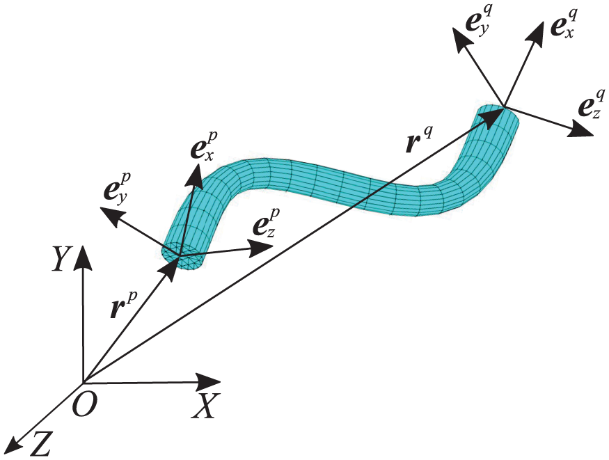
Configuration of the superelement undergoing large displacements and deformations.

The velocity vector can be obtained by differentiating equation (9) with respect to time, as follows

$$\mathit{v}=\{\begin{array}{cccc}{\mathit{v}}^{p\mathbf{T}}\hfill & {\mathbf{\omega }}^{p\mathbf{T}}\hfill & {\mathit{v}}^{q\mathbf{T}}\hfill & {\mathbf{\omega }}^{q\mathbf{T}}\hfill \end{array}{\}}^{\mathbf{T}}$$

(10)

where ${\mathit{v}}^p$ and ${\mathit{v}}^q$ are the absolute nodal translational velocities and ${\mathbf{\omega }}^p$ and ${\mathbf{\omega }}^q$ are absolute nodal rotational velocities.

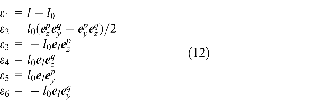
Deformation modes and potential energy

According to Jonker and Meijaard, ²⁵ elastic deformation can be described by a set of deformation coordinates expressed as functions of the nodal coordinates x , as follows

$$\mathbf{\epsilon }\mathbf{=}\mathcal{D}\mathbf{(}\mathit{x}\mathbf{)}$$

(11)

and

$$\begin{array}{c}{\epsilon }_1=l-l_0\hfill \\ \multicolumn{1}{c}{{\epsilon }_2=l_0({\mathit{e}}_z^p{\mathit{e}}_y^q-{\mathit{e}}_y^p{\mathit{e}}_z^q)/2}\\ \multicolumn{1}{c}{{\epsilon }_3=-l_0{\mathit{e}}_l{\mathit{e}}_z^p}\\ \multicolumn{1}{c}{{\epsilon }_4=l_0{\mathit{e}}_l{\mathit{e}}_z^q}\\ \multicolumn{1}{c}{{\epsilon }_5=l_0{\mathit{e}}_l{\mathit{e}}_y^p}\\ \multicolumn{1}{c}{{\epsilon }_6=-l_0{\mathit{e}}_l{\mathit{e}}_y^q}\end{array}$$

(12)

where $l_0$ is the reference length of the superelement, $\mathit{l}={\mathit{r}}^q-{\mathit{r}}^p$ is a vector from the boundary node p to q and $l=\parallel \mathit{l}\parallel$ is the distance between the boundary nodes. Vector ${\mathit{e}}_l=({\mathit{r}}^q-{\mathit{r}}^p)/(\Vert {\mathit{r}}^q-{\mathit{r}}^p\Vert )$ is unit in length and pointing from p towards q. The deformation coordinate ${\epsilon }_1$ describes axial deformation, ${\epsilon }_2$ describes torsion and ${\epsilon }_3$ , ${\epsilon }_4$ , ${\epsilon }_5$ and ${\epsilon }_6$ describe bending deformations. These definitions are illustrated in Figure 4.

Figure 4.

Visualisation of the definition of deformation coordinates.

To determine the elastic forces for the superelement, an energy approach can be used. To this end, the relationship between $\epsilon$ and ${\mu }^e$ needs to be defined by using the definition of the deformation coordinates (equation (11)) and the elastic deformation of the linear superelement (equation (6)), as follows

$${\mathit{\mu }}^e=\mathit{A}\mathbf{\epsilon }$$

(13)

where $\mathit{A}=\mathrm{diag}(1,(1/l_0),-(1/l_0),(1/l_0),-(1/l_0),(1/l_0))$ . Here, matrix A describes the relationship between the deformation coordinates defined in equation (12) (Figure 4) and their corresponding constraint modes defined in equation (7) (Figure 2). Using equations (7) and (13), the potential energy of the nonlinear superelement can be written as

$$\begin{array}{c}P=\frac{1}{2}\{\begin{array}{cc}{\mathbf{\mu }}^{e\mathbf{T}}\hfill & {\mathit{\eta }}^{\mathbf{T}}\hfill \end{array}\}\overline{\mathit{S}}\left\{\begin{array}{c}{\mathbf{\mu }}^e\hfill \\ \multicolumn{1}{c}{\mathit{\eta }}\end{array}\right\}\hfill \\ \multicolumn{1}{c}{=\frac{1}{2}\{\begin{array}{cc}{\mathbf{\epsilon }}^{\mathbf{T}}\hfill & {\mathit{\eta }}^{\mathbf{T}}\hfill \end{array}\}{\left[\begin{array}{cc}\mathit{A}\hfill & \hfill \\ \multicolumn{1}{c}{}& \mathbf{I}\hfill \end{array}\right]}^{\mathbf{T}}\overline{\mathit{S}}\left[\begin{array}{cc}\mathit{A}\hfill & \hfill \\ \multicolumn{1}{c}{}& \mathbf{I}\hfill \end{array}\right]\left\{\begin{array}{c}\mathbf{\epsilon }\hfill \\ \multicolumn{1}{c}{\mathit{\eta }}\end{array}\right\}}\\ \multicolumn{1}{c}{=\frac{1}{2}\{\begin{array}{cc}{\mathbf{\epsilon }}^{\mathbf{T}}\hfill & {\mathit{\eta }}^{\mathbf{T}}\hfill \end{array}\}\tilde{\mathit{S}}\left\{\begin{array}{c}\mathbf{\epsilon }\hfill \\ \multicolumn{1}{c}{\mathit{\eta }}\end{array}\right\}}\end{array}$$

(14)

The equivalent stiffness matrix of the nonlinear superelement is

$$\tilde{\mathit{S}}={\left[\begin{array}{cc}\mathit{A}\hfill & \hfill \\ \multicolumn{1}{c}{}& \mathbf{I}\hfill \end{array}\right]}^{\mathbf{T}}\overline{\mathit{S}}\left[\begin{array}{cc}\mathit{A}\hfill & \hfill \\ \multicolumn{1}{c}{}& \mathbf{I}\hfill \end{array}\right]$$

(15)

Kinetic energy

Similarly to the potential energy, the kinetic energy of the nonlinear superelement can be obtained by relating the absolute velocity vector v to the velocity vector $\overline{\mathit{v}}$ , which is defined with respect to the local reference coordinate frame. This requires relating the derivatives of nodal coordinates $\stackrel{·}{\mathit{x}}$ to the derivatives of reduced coordinates $\stackrel{·}{\mathbf{\mu }}$ . The relationship between v and $\overline{\mathit{v}}$ can be written as

$$\overline{\mathit{v}}={\mathit{B}}_i\mathit{v}$$

(16)

where ${\mathit{B}}_i$ is the velocity transformation matrix. Two approaches can be used for expressing the absolute velocity. In the first approach, the translational and rotational velocities of boundaries p and q are both expressed in a coordinate frame attached to boundary node p. The transformation matrix in this case is

$${\mathit{B}}_1=\left[\begin{array}{cccc}{\mathit{R}}^{e\mathbf{T}}{\mathit{R}}^{p\mathbf{T}}\hfill & \hfill & \hfill & \hfill \\ \multicolumn{1}{c}{}& {\mathit{R}}^{e\mathbf{T}}{\mathit{R}}^{p\mathbf{T}}\hfill & \hfill & \hfill \\ \multicolumn{1}{c}{}& \hfill & {\mathit{R}}^{e\mathbf{T}}{\mathit{R}}^{p\mathbf{T}}\hfill & \hfill \\ \multicolumn{1}{c}{}& \hfill & \hfill & {\mathit{R}}^{e\mathbf{T}}{\mathit{R}}^{p\mathbf{T}}\hfill \end{array}\right]$$

(17)

In the second approach, the translational and rotational velocities of boundary p are expressed in a coordinate frame attached to boundary node p, while the velocities of boundary q are expressed in a coordinate frame attached to boundary node q. The transformation matrix in this scenario is

$${\mathit{B}}_2=\left[\begin{array}{cccc}{\mathit{R}}^{e\mathbf{T}}{\mathit{R}}^{p\mathbf{T}}\hfill & \hfill & \hfill & \hfill \\ \multicolumn{1}{c}{}& {\mathit{R}}^{e\mathbf{T}}{\mathit{R}}^{p\mathbf{T}}\hfill & \hfill & \hfill \\ \multicolumn{1}{c}{}& \hfill & {\mathit{R}}^{e\mathbf{T}}{\mathit{R}}^{q\mathbf{T}}\hfill & \hfill \\ \multicolumn{1}{c}{}& \hfill & \hfill & {\mathit{R}}^{e\mathbf{T}}{\mathit{R}}^{q\mathbf{T}}\hfill \end{array}\right]$$

(18)

The equivalent kinetic energy of the nonlinear superelement can be rewritten as

$$\begin{array}{c}T=\frac{1}{2}{\overline{\mathit{v}}}^{\mathbf{T}}\overline{\mathit{M}}\overline{\mathit{v}}\hfill \\ \multicolumn{1}{c}{=\frac{1}{2}\{\begin{array}{cc}{\stackrel{·}{\mathit{x}}}^{\mathbf{T}}\hfill & {\stackrel{·}{\mathit{\eta }}}^{\mathbf{T}}\hfill \end{array}\}{\left[\begin{array}{cc}{\mathbf{B}}_i\hfill & \hfill \\ \multicolumn{1}{c}{}& \mathbf{I}\hfill \end{array}\right]}^{\mathbf{T}}\overline{\mathit{M}}\left[\begin{array}{cc}{\mathbf{B}}_i\hfill & \hfill \\ \multicolumn{1}{c}{}& \mathbf{I}\hfill \end{array}\right]\left\{\begin{array}{c}\stackrel{·}{\mathbf{x}}\hfill \\ \multicolumn{1}{c}{\stackrel{·}{}\mathit{\eta }}\end{array}\right\}}\\ \multicolumn{1}{c}{=\frac{1}{2}\{\begin{array}{cc}{\stackrel{·}{\mathit{x}}}^{\mathbf{T}}\hfill & {\stackrel{·}{\mathit{\eta }}}^{\mathbf{T}}\hfill \end{array}\}\tilde{\mathit{M}}\left\{\begin{array}{c}\stackrel{·}{\mathit{x}}\hfill \\ \multicolumn{1}{c}{\stackrel{·}{\mathit{\eta }}}\end{array}\right\}}\end{array}$$

(19)

The mass matrix of the nonlinear superelement can be written as

$$\tilde{\mathit{M}}={\left[\begin{array}{cc}{\mathit{B}}_i\hfill & \hfill \\ \multicolumn{1}{c}{}& \mathbf{I}\hfill \end{array}\right]}^{\mathbf{T}}\overline{\mathit{M}}\left[\begin{array}{cc}{\mathit{B}}_i\hfill & \hfill \\ \multicolumn{1}{c}{}& \mathbf{I}\hfill \end{array}\right]$$

(20)

Dynamics

The equations of motion for the nonlinear superelement can be written as

$$\tilde{\mathit{M}}\left\{\begin{array}{c}\stackrel{··}{\mathit{x}}\hfill \\ \multicolumn{1}{c}{\stackrel{··}{\mathit{\eta }}}\end{array}\right\}+\tilde{\mathit{G}}\left\{\begin{array}{c}\stackrel{·}{\mathit{x}}\hfill \\ \multicolumn{1}{c}{\stackrel{·}{\mathit{\eta }}}\end{array}\right\}={\mathit{f}}_{\mathrm{ext}}-{\mathit{f}}_{\mathrm{in}}$$

(21)

where $\tilde{\mathit{G}}$ is the velocity-related gyroscopic matrix of the nonlinear superelement and ${\mathit{f}}_{\mathrm{in}}$ is the vector of elastic forces. The components can be written as

$$\begin{array}{c}\tilde{\mathit{G}}={\left[\begin{array}{cc}{\stackrel{·}{\mathit{B}}}_i\hfill & \hfill \\ \multicolumn{1}{c}{}& 0\hfill \end{array}\right]}^{\mathbf{T}}\overline{\mathit{M}}\left[\begin{array}{cc}{\mathit{B}}_i\hfill & \hfill \\ \multicolumn{1}{c}{}& \mathbf{I}\hfill \end{array}\right]+{\left[\begin{array}{cc}{\mathit{B}}_i\hfill & \hfill \\ \multicolumn{1}{c}{}& \mathbf{I}\hfill \end{array}\right]}^{\mathbf{T}}\overline{\mathit{M}}\left[\begin{array}{cc}{\stackrel{·}{\mathit{B}}}_i\hfill & \hfill \\ \multicolumn{1}{c}{}& 0\hfill \end{array}\right]\hfill \\ \multicolumn{1}{c}{+{\mathit{B}}_i^{*\mathbf{T}}\overline{\mathit{M}}\left[\begin{array}{cc}{\mathit{B}}_i\hfill & \hfill \\ \multicolumn{1}{c}{}& \mathbf{I}\hfill \end{array}\right]}\\ \multicolumn{1}{c}{{\mathit{f}}_{\mathrm{in}}=\left[\begin{array}{cc}\frac{\partial \mathbf{\epsilon }}{\partial \mathit{x}}\hfill & \hfill \\ \multicolumn{1}{c}{}& \mathbf{I}\hfill \end{array}\right]\mathit{S}\mathbf{\epsilon }}\end{array}$$

(22)

where ${\mathit{B}}_i^{*}=(\partial \overline{\mathit{v}})/(\partial (\mathit{x},\mathit{\eta }))$ .

Quadratic 3D ANCF beam element

This section briefly reviews the quadratic ANCF beam element used in this article. Subsequently, the gyroscopic matrix, which is necessary for computing the Campbell diagram, is introduced.

The beam element used is a 3D and three-noded element. ²⁸ As shown in Figure 5, the element is defined by one position vector and two slope vectors at each node.

Figure 5.

The geometric description of the ANCF beam element.

Element kinematics

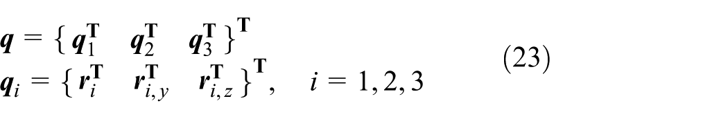
For the quadratic three-node element, the nodal coordinate vector q is defined as

$$\begin{array}{c}\mathit{q}={\{\begin{array}{ccc}{\mathit{q}}_1^{\mathbf{T}}\hfill & {\mathit{q}}_2^{\mathbf{T}}\hfill & {\mathit{q}}_3^{\mathbf{T}}\hfill \end{array}\}}^{\mathbf{T}}\hfill \\ \multicolumn{1}{c}{{\mathit{q}}_i={\{\begin{array}{ccc}{\mathit{r}}_i^{\mathbf{T}}\hfill & {\mathit{r}}_{i,y}^{\mathbf{T}}\hfill & {\mathit{r}}_{i,z}^{\mathbf{T}}\hfill \end{array}\}}^{\mathbf{T}},i=1,2,3}\end{array}$$

(23)

where ${\mathit{r}}_{i,y}$ and ${\mathit{r}}_{i,z}$ are the transverse gradient vectors. The element consists of 27 DOFs. Using these nodal coordinates, the position vector of an arbitrary point within the element is described as

$$\mathit{r}(x,y,z)=\mathit{Sq}$$

(24)

where $\mathit{S}=[S_1\mathbf{I}\dots S_9\mathbf{I}]$ is the shape function matrix, and $x,y,z$ are the coordinates in the element local coordinate system; $x\in [-(L/2),(L/2)]$ indicates the lengthwise direction. The element’s shape functions $S_1,\dots ,S_9$ can be written as follows

$$\begin{array}{c}{S}_1(x)=-\frac{2}{L^2}x(\frac{L}{2}-x)\hfill \\ \multicolumn{1}{c}{S_2(x,y)=y{S}_1,S_3(x,z)=z{S}_1}\\ \multicolumn{1}{c}{S_4(x)=+\frac{2}{L^2}x(\frac{L}{2}+x)}\\ \multicolumn{1}{c}{S_5(x,y)=y{S}_4,S_6(x,z)=z{S}_4}\\ \multicolumn{1}{c}{S_7(x)=-\frac{4}{L^2}(x-\frac{L}{2})(x+\frac{L}{2})}\\ \multicolumn{1}{c}{S_8(x,y)=y{S}_7,S_9(x,z)=z{S}_7}\end{array}$$

(25)

Element strains: structural mechanics formulation

Using the structural mechanics–based approach, strain energy can be expressed as follows

$$\begin{array}{c}\multicolumn{1}{c}{U_{\mathrm{SMF}}=\frac{1}{2}\underset{-L/2}{\overset{L/2}{\int }}(\mathrm{EA}{\mathrm{\Gamma }}_1^2+\mathrm{GA}{k}_2{\mathrm{\Gamma }}_2^2+\mathrm{GA}{k}_3{\mathrm{\Gamma }}_3^2}\\ +\mathrm{GJ}{k}_t{\kappa }_1^2+E{I}_2{\kappa }_2^2+E{I}_3{\kappa }_3^2)\mathrm{d}x\hfill \end{array}$$

(26)

where $k_2$ and $k_3$ are the shear correction factors that are used to obtain the correct shear strain energy. ${\mathrm{\Gamma }}_1,\dots ,{\mathrm{\Gamma }}_3$ and ${\kappa }_1,\dots ,{\kappa }_3$ are the generalised strains, which can be defined using a cross-sectional reference frame. The reference frame can, in turn, be defined using the base vectors ${\mathit{e}}_1,\dots ,{\mathit{e}}_3$ . The unit vectors are described by Nachbagauer et al. ²⁸ as follows

$$\begin{array}{cc}{\mathit{e}}_1=\frac{{\overline{\mathit{e}}}_1}{|{\overline{\mathit{e}}}_1|},\hfill & {\overline{\mathit{e}}}_1={\mathit{r}}_y\times {\mathit{r}}_z\hfill \\ \multicolumn{1}{c}{{\mathit{e}}_3=\frac{{\overline{\mathit{e}}}_3}{|{\overline{\mathit{e}}}_3|},}& {\overline{\mathit{e}}}_3={\mathit{r}}_z\hfill \\ \multicolumn{1}{c}{{\mathit{e}}_2=\frac{{\overline{\mathit{e}}}_2}{|{\overline{\mathit{e}}}_2|},}& {\overline{\mathit{e}}}_2={\overline{\mathit{e}}}_3\times {\overline{\mathit{e}}}_1\hfill \end{array}$$

(27)

The generalised axial strain ${\mathrm{\Gamma }}_1$ and shear strains ${\mathrm{\Gamma }}_2$ and ${\mathrm{\Gamma }}_3$ can now be defined as

$$\begin{array}{c}{\mathrm{\Gamma }}_1={\mathit{e}}_1^{\mathbf{T}}{\mathit{r}}_x-1\hfill \\ \multicolumn{1}{c}{{\mathrm{\Gamma }}_2={\mathit{e}}_2^{\mathbf{T}}{\mathit{r}}_x}\\ \multicolumn{1}{c}{{\mathrm{\Gamma }}_3={\mathit{e}}_3^{\mathbf{T}}{\mathit{r}}_x}\end{array}$$

(28)

where the subscript x indicates length derivatives. Following this, the vector of twist and curvature k can be written as

$$\mathit{k}=\frac{1}{2}\sum _{i=1}^3{\mathit{e}}_i\times {\mathit{e}}_{i,x}=\frac{1}{2}({\mathit{e}}_1\times \mathit{e}{\prime }_{1,x}+{\mathit{e}}_2\times \mathit{e}{\prime }_{2,x}+{\mathit{e}}_3\times \mathit{e}{\prime }_{3,x})$$

(29)

The generalised torsion strain ${\kappa }_1$ and bending strains ${\kappa }_2$ and ${\kappa }_3$ are defined as

$$\begin{array}{c}\mathit{\kappa }={\mathit{A}}_e^{\mathbf{T}}\mathit{k}\hfill \end{array}$$

(30)

where ${\mathit{A}}_e=[\begin{array}{ccc}{\mathit{e}}_1\hfill & {\mathit{e}}_2\hfill & {\mathit{e}}_3\hfill \end{array}]$ is an orthogonal rotation matrix describing the local element coordinate system. In addition to equation (26), a second strain energy term can be used to take into account cross-sectional deformation (without the Poisson effect), defined as follows

$$U_{\mathrm{CSD}}=\frac{1}{2}\underset{-L/2}{\overset{L/2}{\int }}(\mathrm{EA}(E_{\mathrm{yy}}^2+E_{\mathrm{zz}}^2)+{\mathrm{GAE}}_{\mathrm{yz}}^2)\mathrm{d}x$$

(31)

where the strains $E_{\mathrm{yy}}$ , $E_{\mathrm{zz}}$ and $E_{\mathrm{yz}}$ are the components of the Green–Lagrange strain tensor, defined as

$$\begin{array}{c}{E}_{\mathrm{yy}}=\frac{1}{2}({\mathit{r}}_y^{\mathbf{T}}{\mathit{r}}_y-1)\hfill \\ \multicolumn{1}{c}{E_{\mathrm{zz}}=\frac{1}{2}({\mathit{r}}_z^{\mathbf{T}}{\mathit{r}}_z-1)}\\ \multicolumn{1}{c}{E_{\mathrm{yz}}=\frac{1}{2}{\mathit{r}}_y^{\mathbf{T}}{\mathit{r}}_z}\end{array}$$

(32)

Linear dynamics: gyroscopic matrix

For the purposes of transient analysis, the inertia for the ANCF beam element can be simply calculated from the expression of kinetic energy $T=(1/2){\int }_V{\left|\stackrel{·}{\mathit{r}}\right|}^2\mathrm{dm}$ . However, for the linearised eigenvalue solution required in the Campbell diagram computation, a gyroscopic matrix from the system is needed. To this end, small deformations and constant rotational speed $\mathbf{\Omega }$ around the element’s longitudinal axis are assumed. The rotation causes a tangential velocity component ${\mathit{v}}_{\mathbf{\Omega }}(y,z)$ on each point of the element cross section, which is further illustrated in Figure 6.

Figure 6.

The velocity caused by rotation of the ANCF beam element.

Separating the rotational velocity component and using the previously defined orthogonal rotation matrix ${\mathit{A}}_e$ , the velocity of an arbitrary point within the element can be written as

$$\stackrel{·}{\mathit{r}}(x,y,z)=\mathit{v}+{\mathit{v}}_{\mathbf{\Omega }}=\mathit{v}+\mathbf{\Omega }{\mathit{A}}_e\mathit{b}$$

(33)

where v is the velocity of the point without the rotation and vector $\mathit{b}=[0-zy{]}^{\mathbf{T}}$ represents the direction of the rotational velocity component in the cross-sectional frame according to the right-hand rule. In this linearised case, the approximation ${\mathit{A}}_e\approx [\begin{array}{ccc}{\mathit{r}}_x\hfill & {\mathit{r}}_y\hfill & {\mathit{r}}_z\hfill \end{array}]$ is adopted for the rotation matrix. Subsequently, the total kinetic energy of the element (with $\mathrm{d}m=\rho \mathrm{d}V$ ) can be written as

$$T=\frac{1}{2}\underset{V}{\int }{\left|\stackrel{·}{\mathit{r}}\right|}^2\mathrm{d}m=\frac{1}{2}\underset{V}{\int }{\stackrel{·}{\mathit{r}}}^{\mathbf{T}}\stackrel{·}{\mathit{r}}\mathrm{d}m$$

(34)

Substituting equation (33) into equation (34), the kinetic energy can be separated into three terms

$$\begin{array}{l}{T}_1=\frac{1}{2}{\displaystyle \underset{V}{\int }{\mathit{v}}^{\mathit{T}}\mathit{v}}\mathrm{d}m,\hfill \\ T_2=\Omega {\displaystyle \underset{V}{\int }{\mathit{v}}^T{\mathit{A}}_e\mathit{b}}\mathrm{d}m,\hfill \\ T_3=\frac{1}{2}{\Omega }^2{\displaystyle \underset{V}{\int }{\mathit{b}}^T\mathit{b}}\mathrm{d}m\hfill \end{array}$$

(35)

When considering the contributions of these energy terms to the equations of motion, it is apparent that the first term involves translational inertia and results in the mass matrix. The second term involves the gyroscopic effect and results in the gyroscopic matrix. The third and final term, a constant term that represents rotational inertia, does not contribute to the linearised equations of motion used in the eigenvalue analysis. Using the definitions $\mathit{v}=\mathit{S}\stackrel{·}{\mathit{q}}$ , ${\mathit{r}}_y={\mathit{S}}_y\mathit{q}$ and ${\mathit{r}}_z={\mathit{S}}_z\mathit{q}$ , the mass matrix and gyroscopic matrix can be written, correspondingly, as follows

$$\mathit{M}=\underset{V}{\int }{\mathit{S}}^{\mathbf{T}}\mathit{S}\mathrm{d}m,\mathit{G}=2\underset{V}{\int }{\mathit{S}}^{\mathbf{T}}(y{\mathit{S}}_z-z{\mathit{S}}_y)\mathrm{d}m$$

(36)

Taking damping into account, the resulting linearised system of equations of motion is of the form

$$\mathit{M}\stackrel{··}{\mathit{q}}+(\mathbf{\Omega }\mathit{G}+\mathit{C})\stackrel{·}{\mathit{q}}+\mathit{Kq}={\mathit{f}}_{\mathrm{ext}}$$

(37)

Numerical examples

In this section, the two-node superelement and the three-node ANCF beam element are used in numerical simulation examples. The first example case is a spinning beam undergoing large rotations, while the second is a complex-shaped flexible rotor with an unbalanced disc. In addition to computing the start-up response, which is done in both examples, the critical speeds of the system are analysed in the second example. Reference results for both cases are produced using the commercial FE software ANSYS.

Spinning beam

In this section, the elements are applied to the simple spinning beam example from. ²⁶ A flexible beam, as shown in Figure 7, is connected to the ground via a revolute joint at one end. The beam accelerates from rest to a constant angular velocity, with the motion described as

$$e(t)=\{\begin{array}{c}\frac{\omega }{T}[\frac{1}{2}{t}^2-\frac{T^2}{4{\pi }^2}(1-\cos \left(\frac{2\pi t}{T}\right))],0\le t\le T\hfill \\ \multicolumn{1}{c}{\omega (t-\frac{1}{2}T),t>T}\end{array}$$

(38)

where $\omega$ is the final angular velocity and $T=15\mathrm{s}$ is the spin-up time. As shown in Figure 7, two load cases with different constant angular velocities are considered, case 1 being $\omega =4\mathrm{rad}/\mathrm{s}$ and case 2 being $\omega =8\mathrm{rad}/\mathrm{s}$ . The cross-sectional dimensions and material properties are shown in Table 1. The flexible beam is discretised using four superelements built based on a linear FE model created using 300 SOLID186 elements in ANSYS. This FE model has 1935 nodes in total. A reference solution is provided using ANSYS with 20 BEAM188 elements, which is a nonlinear Timoshenko-based beam element. The total simulation time was 20 s, during which the transverse deformation of the free end was recorded.

Figure 7.

Sketch of spinning beam and its prescribed motion.

Table 1.

Parameters for spinning beam.

Length	Height	Width	Density	Young’s modulus	Poisson’s ratio
L	H	W	$\rho$	E	v
8 m	0.03675 m	0.001986 m	2766 kg/m3	6.895 ×1010 Pa	0.3

The ANCF beam element model was computed in MATLAB using the solver ‘radau5’ (implicit Runge–Kutta method of order 5) with Newton’s method for nonlinear solution. The relative and absolute tolerances were 1e−4 and 1e−6, respectively. The elastic forces were integrated using a two-point Gauss quadrature lengthwise and three-point Lobatto quadratures laterally. The results based on the superelement with both transformation matrices $B1$ and $B2$ are compared with the reference solution in Figure 8.

Figure 8.

Spinning beam free-end deformation Δy ( 20 BEAM188 elements, 4 nonlinear superelements with velocity transformation matrix B1, 4 nonlinear superelements with velocity transformation matrix $B2$ , 16 ANCF beam elements).

Figure 8 shows that superelements with either transformation matrix give nearly identical results in the simulation. However, while in case 1 the results of the superelements are in very good agreement with the reference, in case 2 the difference is noticeable. The difference is due to the increase in nonlinear effects caused by the higher angular velocity in case 2. For higher velocities, the linear assumption is no longer adequate and the response becomes unstable. This was also reported in Cardona and Géradin ²¹ and Bauchau and Rodriguez ²² The results of the ANCF element follow the reference set closely in the lower speed case, but also show a difference in the higher speed case.

Rotor with unbalanced disc

In this section, the superelement and the nonlinear ANCF beam element are applied to a rotor dynamics problem. A rotor system with an unbalanced disc, which was originally proposed in Bauchau et al. ²⁹ as a benchmark problem, is chosen as an example case. The rotor system is supported at its ends by bearings, as shown in Figure 9(a). At point R, the shaft is connected to the ground by means of a revolute joint. At point T, the shaft is connected to the ground via a cylindrical joint. A rigid disc is attached to the shaft at its mid-span, and the centre of the disc is located above the shaft centre by distance d, thereby creating an unbalance in the system. The geometric parameters of the rotor system are shown in Table 2. First, the superelement and the ANCF beam element were used in modal analysis. The Campbell diagram, which shows the variation in the rotor’s natural frequencies with respect to its rotating speed, was computed. After this phase, a transient simulation was performed. In the transient simulation, the motion of the revolute joint at point R was prescribed as follows

$$\Omega (t)=\{\begin{array}{cc}{A}_1\omega \left(1-\cos \left(\frac{\pi t}{T_1}\right)\right)/2,\hfill & 0\le t\le T_1\hfill \\ A_1\omega ,\hfill & T_1\mathrm{<}t\le T_2\hfill \\ A_1\omega +(A_2-A_1)\omega \left[1-\cos \left(\frac{\pi (t-T_2)}{T_3-T_2}\right)\right]/2,\hfill & T_2\mathrm{<}t\le T_3\hfill \\ A_2\omega ,\hfill & t>T_3\hfill \end{array}$$

(39)

where $A_1=0.8$ , $A_2=1.2$ , $T_1=0.5\mathrm{s}$ , $T_2=1\mathrm{s}$ , $T_3=1.25\mathrm{s}$ and $\omega =60\mathrm{rad}/\mathrm{s}$ . This prescribed motion is further illustrated in Figure 9(b).

Figure 9.

Sketch of the rotor system and its motion.

Table 2.

Parameters of the rotor system.

Physical properties	Parameter	Symbol	Value
	Density	$\rho$	7800 kg/m3
	Young’s modulus	E	$2.1\times {10}^{11}\mathrm{Pa}$
	Poisson’s ratio	$\nu$	$0.3$
	Gravity	g	9.81 m/s2
System geometry	Shaft length	L	6 m
	Shaft inner radius	$R_i$	0.045 m
	Shaft outer radius	$R_o$	0.05 m
	Disc radius	$R_d$	0.24 m
	Disc thickness	$t_d$	0.05 m
	Disc offset	d	0.05 m
System stiffness	Axial	S	313.4 MN
	Shearing	$K_{22}$	60.5 MN
	Shearing	$K_{33}$	60.5 MN
	Torsional	$H_{11}$	272.7 kN m2
	Bending	$H_{22}$	354.5 kN m2
	Bending	$H_{33}$	354.5 kN m2

In rotor dynamics applications, the natural frequencies and excitation frequencies of the rotor-bearing system are often dependent on the rotational speed of the rotor. Usually, the natural frequencies are presented as a function of the rotation speed in the so-called Campbell diagram, from which it is possible to detect the critical rotating speeds of the system. To provide a reference solution, the rotor was modelled in ANSYS with a large number of SOLID186 elements, and a modal analysis was performed with gyroscopic effects included. During the analysis, the studied rotational speed range was from 0 to 10,000 r/min. As it is difficult to exactly model the behaviour of idealised revolute and cylinder joints in a solid element model, all the DOFs on the boundary nodes were constrained in the case of element SOLID186.

First, the natural frequencies of the rotor system were computed using the linear superelement. The mass matrix, stiffness matrix and gyroscopic matrix from the original FE model were reduced by 12 constraint modes and 10 clamped interface normal modes. The Campbell diagram based on the linear superelement was compared with the corresponding original SOLID186 model as well as a tranditional beam element model (BEAM188). A comparison between the linear superelement and SOLID186 is shown in Figure 10. It can be observed that the linear superelement agrees with the original model well.

Figure 10.

Campbell diagram based on SOLID186 and 1 linear superelement, clamped-clamped boundary condition ( large number of SOLID186 elements, 1 linear superelement with 10 normal modes). Dashed diagonal line represents spin frequency.

According to the authors’ knowledge, only linear theory was used when determining natural frequencies in previous publications. It is questionable whether linear theory is adequate for modal problems. It is also necessary to clarify how to use nonlinear theory in modal analysis and how nonlinear effects affect natural frequencies. For these purposes, the nonlinear superelement and the nonlinear ANCF beam element were used in the computation of the Campbell diagram of the rotor system.

When using the nonlinear superelement, the stiffness matrix was calculated with the finite difference method from the elastic force vector $f_{\mathrm{in}}$ in equation (22). Since the mass matrix and the velocity-related gyroscopic matrix were uncoupled from each other, the modal analysis of the superelement can be taken as a quadratic eigenvalue problem which is similar to linear modal analysis, while the matrices have a nonlinear relationship with the velocity vectors. The rotor was meshed with four nonlinear superelements as shown in Figure 11. The first and the fourth superelements are built based on substructure 1, while the second and third superelements are built based on substructures 2 and 3, respectively. The stiffness matrix for the ANCF beam element was also calculated using finite differences. Again, the elastic forces were integrated using a two-point Gauss quadrature lengthwise and three-point Lobatto quadratures laterally.

Figure 11.

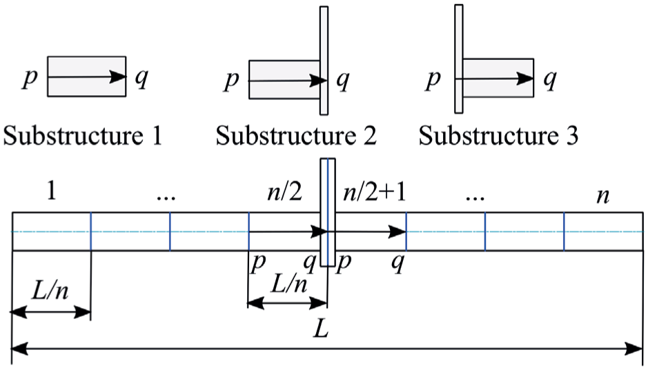
Discretisation of the rotor system.

The Campbell diagrams based on the nonlinear superelement and ANCF beam element are shown in Figure 12. Figure 12 shows that the results based on eight ANCF beam elements are nearly identical to the ANSYS results, whereas the nonlinear superelement does not agree with the reference solution well. The nonlinear superelement only gives the correct solutions for the first bending modes.

Figure 12.

Campbell diagram based on nonlinear superelement and ANCF beam element in comparison with ANSYS BEAM188, revolute-cylinder joint boundary condition ( 20 BEAM188 elements, 4 ANCF beam elements, 4 nonlinear superelements). Dashed diagonal line represents spin frequency.

Second, the nonlinear superelement and the ANCF beam element were used to simulate the transient response of the system. The rotor shaft starts to rotate from static equilibrium under gravity load. The prescribed angular velocity described in equation (39) is applied and the transient response is analysed in the time range $t=[0,2.5]\mathrm{s}$ . According to previously presented results, the first $1\times$ critical speed of the rotor is approximately 550.6 r/min or 57.66 rad/s. As the shaft accelerates, it passes the first critical speed of the system and the operation goes from sub-critical to super-critical. During the simulation, the displacement of the mid-span point was investigated. The rotor was meshed with four superelements and the velocity transformation matrix $B2$ was used. The results presented in Bauchau et al., ²⁹ designated ‘Dymore’, were used as a reference.

The ANCF beam element model was computed in MATLAB using the solver ‘radau5’ (implicit Runge–Kutta method of order 5) with Newton’s method for nonlinear solution, as in the previous example. The relative and absolute tolerances were 1e−4 and 1e−6, respectively. The elastic forces were integrated using a two-point Gauss quadrature lengthwise and three-point Lobatto quadratures laterally.

The displacements along the directions of ${\overline{i}}_2$ and ${\overline{i}}_3$ are presented in Figure 13, designated $u_2$ and $u_3$ , respectively. As can be seen, the results based on ANCF beam elements agree well with the reference solution. While the results based on the superelement also agree with the reference, they do not follow the reference as accurately as the ANCF beam results. The errors visible in the response given by the superelement solution increase as the rotating speed increases. Especially after $t=1.33\mathrm{s}$ , when the rotating speed passes the first critical speed of the rotor system, the superelement results fail to follow the reference.

Figure 13.

Displacement of mid-span point ( Dymore solution, ⁹ 4 nonlinear superelements with velocity transformation matrix $B2$ , 8 ANCF beam elements).

The trajectory of the mid-span point shows the rotor’s dynamic response. The trajectory is presented in both the inertial frame $[\begin{array}{ccc}{\overline{i}}_1\hfill & {\overline{i}}_2\hfill & {\overline{i}}_3\hfill \end{array}]$ and the rotating frame $[\begin{array}{ccc}{\overline{e}}_1\hfill & {\overline{e}}_2\hfill & {\overline{e}}_3\hfill \end{array}]$ in Figure 14. It is apparent that the shaft becomes self-centring when it passes the critical speed. The ANCF beam element–based results are practically identical to the referenced Dymore results. Although the superelement is not as accurate as the ANCF beam element, the difference remains within an acceptable range, and only four elements are enough for an acceptable solution. Therefore, computationally speaking, it seems that the superelement has an edge over the studied ANCF beam element.

Figure 14.

Trajectory of shaft’s mid-span point ( Dymore solution, ⁹ 4 nonlinear superelements with velocity transformation matrix $B2$ , 8 ANCF beam elements).

The transient responses based on different velocity transformation matrices and different numbers of superelements are presented in Figure 15. When using two superelements, the solutions based on velocity transformations $B1$ and $B2$ give roughly the same results. However, these results differ considerably from the reference. When the number of superelements increases, the solutions based of $B1$ and $B2$ diverge. The formulation based on velocity transformation matrix $B1$ fails to follow the reference, while the $B2$ formulation seems to suffer from a convergence problem, as the displacement obtained with eight elements is larger than that obtained with four elements. This may be caused by the sharing of interface modes.

Figure 15.

Trajectory of shaft’s mid-span point, observed in rotating frame ( Dymore solution, ⁹ nonlinear superelement with velocity transformation matrix $B1$ , nonlinear superelement with velocity transformation matrix $B2$ ).

Conclusion

In this article, the superelement formulation as proposed by Boer et al. ²⁶ and the quadratic beam element based on the ANCF as proposed by Nachbagauer et al. ²⁸ were applied to the simulation of high-speed rotating structures. To this end, both element formulations were briefly reviewed by highlighting their distinctive features. The numerical results produced using both formulations were compared against those produced in the commercial FE software ANSYS and those available in literature.

The performance of the studied formulations was examined using two numerical examples in the field of rotating structures. The first test was a spinning beam example in which the transient response was examined using the ANCF-based beam elements and nonlinear superelements. The response was recorded for two rotational speeds. The results show acceptable agreement between all result sets at low speed. Nevertheless, the more pronounced rotational effects cause a divergence at the higher speed.

The second test was an unbalanced rotating shaft example, originally proposed by Bauchau et al., ²⁹ where both modal analysis and transient analysis were performed. Both nonlinear and linear superelements, in addition to the ANCF-based beam element, were used in this test. In this case, both modal and transient results show agreement between the ANSYS model and the ANCF beam model. However, the superelement results were more unpredictable. Although in certain cases the superelements were able to produce acceptable results with lower element numbers compared to the ANCF beam elements, the results based on superelements do not agree with ANSYS results consistently in all cases. This is compounded by the observation that the number of superelements has a seemingly unpredictable effect on the results produced.

Two conclusions can be drawn from these outcomes. The first is that the ANCF-based element seems to produce results that agree with conventional beam elements with minor differences. This holds true even in cases where rotational effects are significant, as evidenced by the results. On the other hand, the second conclusion is that the superelement approach seems to be unable do the same. Especially in the second example, the differences in results are quite significant.

The superelement was expected to improve computational efficiency by producing reliable solutions with just one element since the convergence problem was not discussed in past publications. Generally, when a distributed load is considered, more elements should be meshed to improve the accuracy of the simulation. Accordingly, as shown in the second example, four superelements appear to perform better than two. However, when the element number is increased to eight for more in-depth observation, the convergence problem emerges. One potential reason for this problem is the sharing of deformation at the interface surface of two connected elements. Another is the selection of the reference coordinate frame for calculating the velocity transformation matrix.